VGP assembly pipeline - short version

 Delphine Lariviere
 Alex Ostrovsky
 Cristóbal Gallardo
 Brandon Pickett
 Linelle Abueg
OverviewQuestions:
Objectives:
what combination of tools can produce the highest quality assembly of vertebrate genomes?
How can we evaluate how good it is?
Requirements:
Learn the tools necessary to perform a de novo assembly of a vertebrate genome
Evaluate the quality of the assembly
- Introduction to Galaxy Analyses
- Sequence analysis
- Quality Control: slides slides - tutorial hands-on
Time estimation: 1 hourLevel: Intermediate IntermediateSupporting Materials:Last modification: May 18, 2023License: Tutorial Content is licensed under Creative Commons Attribution 4.0 International License. The GTN Framework is licensed under MITShort Link: https://gxy.io/GTN:T00040
Introduction
The Vertebrate Genome Project (VGP), a project of the Genome 10K (G10K) Consortium, aims to generate high-quality, near error-free, gap-free, chromosome-level, haplotype-phased, annotated reference genome assemblies for every vertebrate species (Rhie et al. 2020). The VGP has developed a fully automated de-novo genome assembly pipeline, which uses a combination of three different technologies: Pacbio high fidelity reads (HiFi), Bionano optical maps, and all-versus-all chromatin conformation capture (Hi-C) data.
As a result of a collaboration with the VGP team, a training including a step-by-step detailed description of parameter choices for each step of assembly was developed for the Galaxy Training Network (Lariviere et al. 2022). The following tutorial instead provides a quick walkthrough on how the workflows can be used to rapidly assemble a genome using the VGP pipeline with the Galaxy Workflow System (GWS).
GWS facilitates analysis repeatability, while minimizing the number of manual steps required to execute an analysis workflow, and automating the process of inputting parameters and software tool version tracking. The objective of this training is to explain how to run the VGP workflow, focusing on what are the required inputs and which outputs are generated and delegating how the steps are executed to the GWS.
AgendaIn this tutorial, we will cover:
Getting started on Galaxy
This tutorial assumes you are comfortable getting data into Galaxy, running jobs, managing history, etc. If you are unfamiliar with Galaxy, we recommed you visit the Galaxy Training Network. Consider starting with the following trainings:
- Introduction to Galaxy
- Galaxy 101
- Getting Data into Galaxy
- Using Dataset Collections
- Introduction to Galaxy Analyses
- Understanding the Galaxy History System
- Downloading and Deleting Data in Galaxy
VGP assembly workflow structure
The VGP assembly pipeline has a modular organization, consisting in five main subworkflows (fig. 1), each one integrated by a series of data manipulation steps. Firstly, it allows the evaluation of intermediate steps, which facilitates the modification of parameters if necessary, without the need to start from the initial stage. Secondly, it allows to adapt the workflow to the available data.
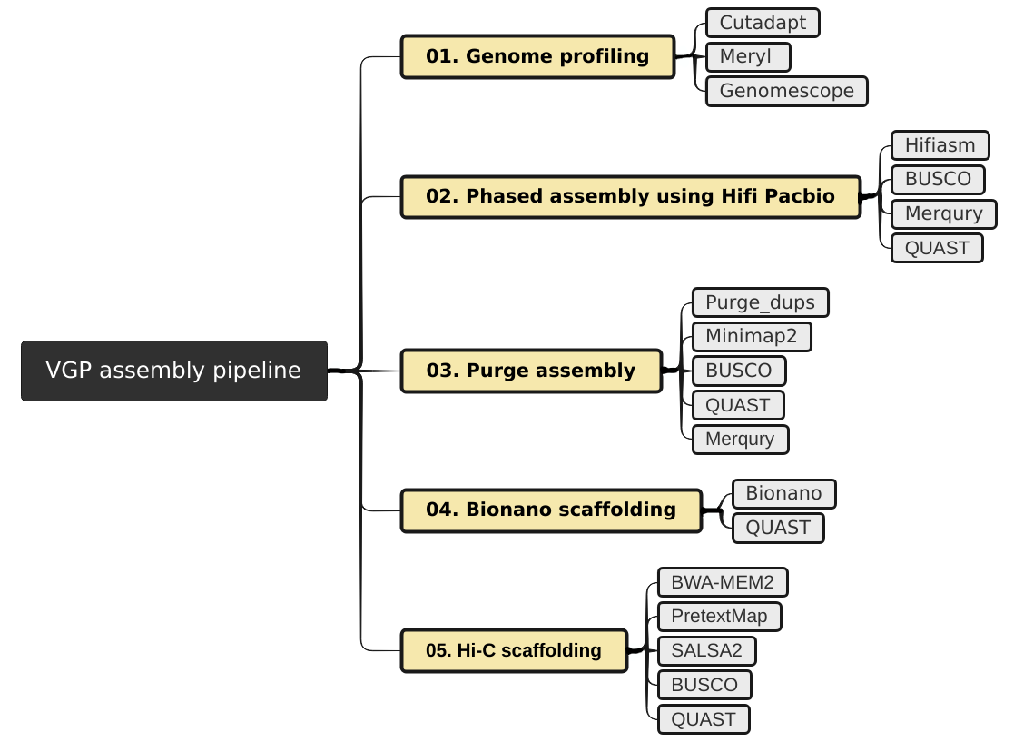
The VGP pipeline first uses an assembly program to generate contiguous sequences in an assembly (contigs). When Hi-C data and Bionano data are avilable, then they are used to generate one or more contigs joined by gap sequence (scaffolds). When both data types are available, then Bionano scaffolding is run first before Hi-C scaffolding, but if optical maps are not available then HiC scaffolding can be run on the contigs.
Comment: Input option orderThis tutorial assumes the input datasets are high-quality. QC on raw read data should be performed before it is used. QC on raw read data is outside the scope of this tutorial.
Get data
For this tutorial, the first step is to get the datasets from Zenodo. The VGP assembly pipeline uses data generated by a variety of technologies, including PacBio HiFi reads, Bionano optical maps, and Hi-C chromatin interaction maps.
Hands-on: Data upload
- Create a new history for this tutorial
Import the files from Zenodo
- Open the file galaxy-upload upload menu
- Click on Rule-based tab
- “Upload data as”:
DatasetsCopy the tabular data, paste it into the textbox and press Build
Hi-C_dataset_F https://zenodo.org/record/5550653/files/SRR7126301_1.fastq.gz?download=1 fastqsanger.gz Hi-C Hi-C_dataset_R https://zenodo.org/record/5550653/files/SRR7126301_2.fastq.gz?download=1 fastqsanger.gz Hi-C Bionano_dataset https://zenodo.org/record/5550653/files/bionano.cmap?download=1 cmap Bionano- From Rules menu select
Add / Modify Column Definitions
- Click
Add Definitionbutton and selectName: columnA- Click
Add Definitionbutton and selectURL: columnB- Click
Add Definitionbutton and selectType: columnC- Click
Add Definitionbutton and selectName Tag: columnD- Click
Applyand press UploadImport the remaining datasets from Zenodo
- Open the file galaxy-upload upload menu
- Click on Rule-based tab
- “Upload data as”:
CollectionsCopy the tabular data, paste it into the textbox and press Build
dataset_01 https://zenodo.org/record/6098306/files/HiFi_synthetic_50x_01.fasta?download=1 fasta HiFi HiFi_collection dataset_02 https://zenodo.org/record/6098306/files/HiFi_synthetic_50x_02.fasta?download=1 fasta HiFi HiFi_collection dataset_03 https://zenodo.org/record/6098306/files/HiFi_synthetic_50x_03.fasta?download=1 fasta HiFi HiFi_collection- From Rules menu select
Add / Modify Column Definitions
- Click
Add Definitionbutton and selectList Identifier(s): columnA- Click
Add Definitionbutton and selectURL: columnB- Click
Add Definitionbutton and selectType: columnC- Click
Add Definitionbutton and selectGroup Tag: columnD- Click
Add Definitionbutton and selectCollection Name: columnE- Click
Applyand press Upload
If working on a genome other than the example yeast genome, you can upload the VGP data from the VGP/Genome Ark AWS S3 bucket as follows:
Hands-on: Import data from GenomeArk
- Open the file galaxy-upload upload menu
- Click on Choose remote files tab
- Click on the Genome Ark button and then click on species
You can find the VGP data following this path:
/species/${Genus}_${species}/${specimen_code}/genomic_data. Inside a given datatype directory (e.g.pacbio), select all the relevant files individually until all the desired files are highlighted and click the Ok button. Note that there may be multiple pages of files listed. Also note that you may not want every file listed.
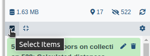
- Click on galaxy-selector Select Items at the top of the history panel
- Check all the datasets in your history you would like to include
Click n of N selected and choose Build Dataset List
- Enter a name for your collection
- Click Create List to build your collection
- Click on the checkmark icon at the top of your history again
Once we have imported the datasets, the next step is to import the VGP workflows from the WorkflowHub.
Import workflows from WorkflowHub
WorkflowHub is a workflow management system which allows workflows to be FAIR (Findable, Accessible, Interoperable, and Reusable), citable, have managed metadata profiles, and be openly available for review and analytics.
Hands-on: Import a workflow
- Click on the Workflow menu, located in the top bar.
- Click on the Import button, located in the right corner.
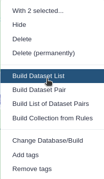
In the section “Import a Workflow from Configured GA4GH Tool Registry Servers (e.g. Dockstore)”, click on Search form.
- In the TRS Server: workflowhub.eu menu you should type
name:vgp- Click on the desired workflow, and finally select the latest available version.
After that, the imported workflows will appear in the main workflow menu. In order to initialize the workflow, we just need to click in the workflow-run Run workflow icon.
The workflows imported are marked with a red square in the following figure:
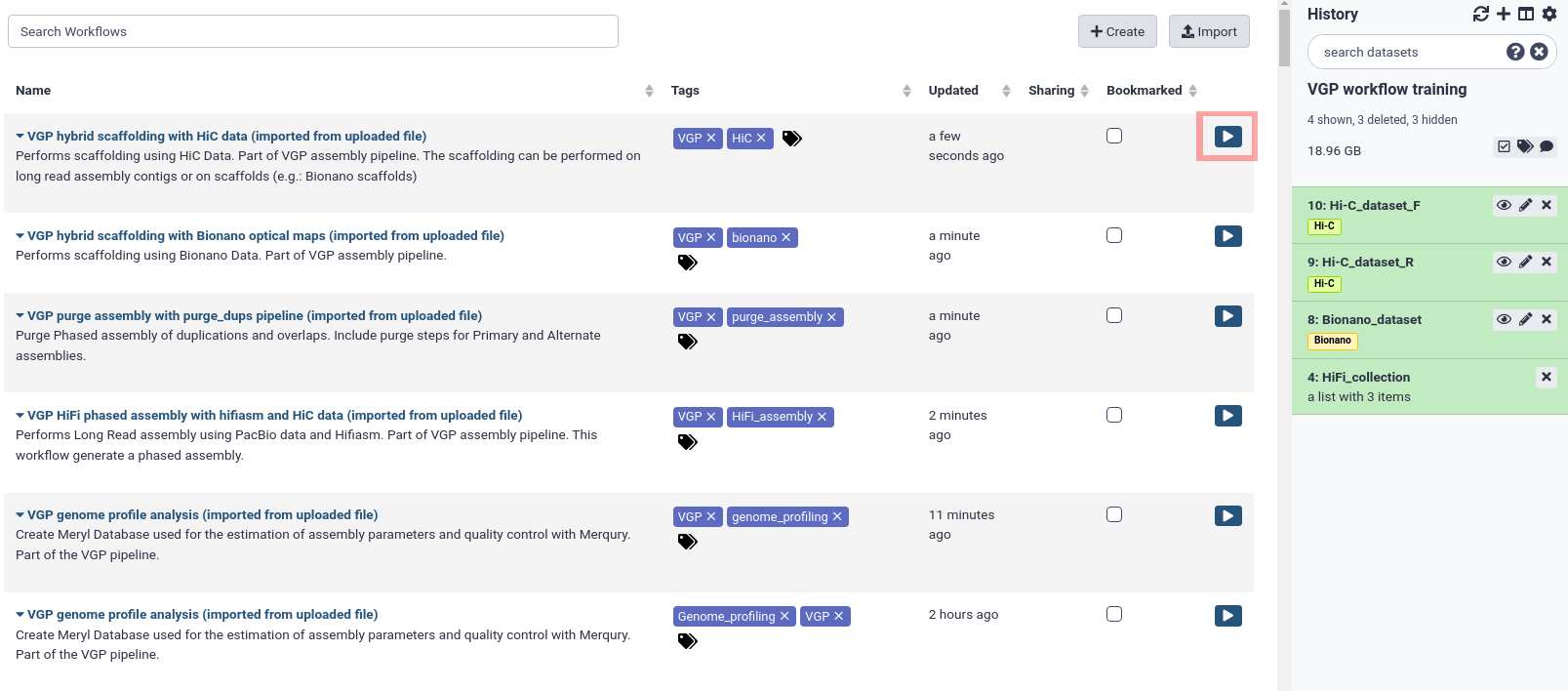
Once we have imported the datasets and the workflows, we can start with the genome assembly.
Comment: Workflow-centric Research ObjectsIn WorkflowHub, workflows are packaged, registered, downloaded and exchanged as Research Objects using the RO-Crate specification, with test and example data, managed metadata profiles, citations and more.
Genome profile analysis
exchange Switch to step by step version
Now that our data and workflows are imported, we can run our first workflow. Before the assembly can be run, we need to collect metrics on the properties of the genome under consideration, such as the expected genome size according to our data. The present pipeline uses Meryl for generating the k-mer database and Genomescope2 for determining genome characteristics based on a k-mer analysis.
Hands-on: VGP genome profile analysis workflow
- Click in the Workflow menu, located in the top bar
- Click in the workflow-run Run workflow buttom corresponding to
VGP genome profile analysis- In the Workflow: VGP genome profile analysis menu:
- param-collection “Collection of Pacbio Data”:
7: HiFi_collection- “K-mer length”:
31- “Ploidy”:
2- Click on the Run workflow buttom
Comment: K-mer lengthIn this tutorial, we are using a k-mer length of 31. This can vary, but the VGP pipeline tends to use a k-mer length of 21, which tends to work well for most mammalian-size genomes. There is more discussion about k-mer length trade-offs in the extended VGP pipeline tutorial.
Once the workflow has finished, we can evaluate the linear plot generated by Genomescope (fig. 3), which includes valuable information such as the observed k-mer profile, fitted models and estimated parameters. This file corresponds to the dataset 26.
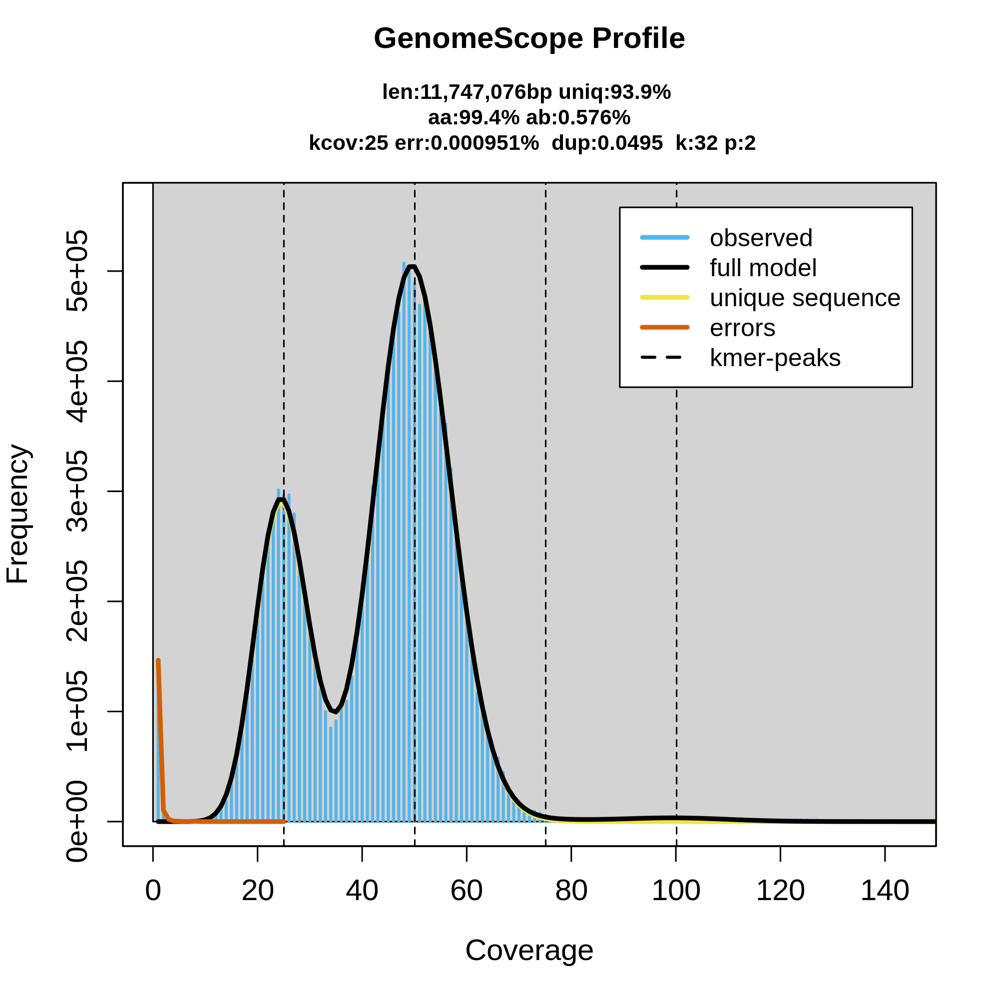
This distribution is the result of the Poisson process underlying the generation of sequencing reads. As we can see, the k-mer profile follows a bimodal distribution, indicative of a diploid genome. The distribution is consistent with the theoretical diploid model (model fit > 93%). Low frequency k-mers are the result of sequencing errors, and are indicated by the red line. GenomeScope2 estimated a haploid genome size of around 11.7 Mbp, a value reasonably close to the Saccharomyces genome size.
Assembly with hifiasm
exchange Switch to step by step version
To generate contigs, the VGP pipeline uses hifiasm. After genome profiling, the next step is to run the VGP HiFi phased assembly with hifiasm and HiC data workflow. This workflow uses hifiasm (HiC mode) to generate HiC-phased haplotypes (hap1 and hap2). This is in contrast to its default mode, which generates primary and alternate pseudohaplotype assemblies. This workflow includes three tools for evaluating assembly quality: gfastats, BUSCO and Merqury.
Hands-on: VGP HiFi phased assembly with hifiasm and HiC data workflow
- Click in the Workflow menu, located in the top bar
- Click in the workflow-run Run workflow buttom corresponding to
VGP HiFi phased assembly with hifiasm and HiC data- In the Workflow: VGP HiFi phased assembly with hifiasm and HiC data menu:
- param-collection “Pacbio Reads Collection”:
7. HiFi_collection- param-file “Meryl database”:
12: Meryl on data 11, data 10, data 9: read-db.meryldb- param-file “HiC forward reads”:
3: Hi-C_dataset_F- param-file “HiC reverse reads”:
2: Hi-C_dataset_R- param-file “Genomescope summary dataset”:
19: Genomescope on data 13 Summary- Click on the Run workflow button
Comment: Input option orderNote that the order of the inputs may differ slightly.
Let’s have a look at the stats generated by gfastats. This output summarizes some main assembly statistics, such as contig number, N50, assembly length, etc.
According to the report, both assemblies are quite similar; the primary assembly includes 18 contigs, whose cumulative length is around 12.2Mbp. The alternate assembly includes 17 contigs, whose total length is 11.3Mbp. As we can see in figure 4a, both assemblies come close to the estimated genome size, which is as expected since we used hifiasm-HiC mode to generate phased assemblies which lowers the chance of false duplications that can inflate assembly size.
Comment: Are you working with pri/alt assemblies?This tutorial uses the hifiasm-HiC workflow, which generates phased hap1 and hap2 assemblies. The phasing helps lower the chance of false duplications, since the phasing information helps the assembler know which genomic variation is heterozygosity at the same locus versus being two different loci entirely. If you are working with primary/alternate assemblies (especially if there is no internal purging in the initial assembly), you can expect higher false duplication rates than we observe here with the yeast HiC hap1/hap2.
Question
- What is the longest contig in the primary assembly? And in the alternate one?
- What is the N50 of the primary assembly?
- Which percentage of reads mapped to each assembly?
- The longest contig in the primary assembly is 1.532.843 bp, and 1.532.843 bp in the alternate assembly.
- The N50 of the primary assembly is 922.430 bp.
- According to the report, 100% of reads mapped to both the primary assembly and the alternate assembly.
Next, we are going to evaluate the outputs generated by BUSCO. This tool provides quantitative assessment of the completeness of a genome assembly in terms of expected gene content. It relies on the analysis of genes that should be present only once in a complete assembly or gene set, while allowing for rare gene duplications or losses (Simão et al. 2015).
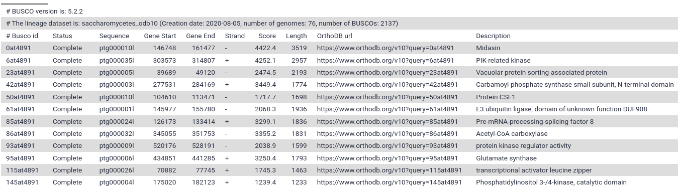
As we can see in the report, the results are simplified into four categories: complete and single-copy, complete and duplicated, fragmented and missing.
Question
- How many complete BUSCO genes have been identified in the primary assembly?
- How many BUSCOs genes are absent?
- According to the report, our assembly contains the complete sequence of 2080 complete BUSCO genes (97.3%).
- 19 BUSCO genes are missing.
Despite BUSCO being robust for species that have been widely studied, it can be inaccurate when the newly assembled genome belongs to a taxonomic group that is not well represented in OrthoDB. Merqury provides a complementary approach for assessing genome assembly quality metrics in a reference-free manner via k-mer copy number analysis. Specifically, it takes our hap1 as the first genome assembly, hap2 as the second genome assembly, and the merylDB generated previously for k-mer counts. Like the other QC metrics we have been looking at, the VGP Hifiasm-HiC workflow will automatically generate the Merqury analysis.
By default, Merqury generates three collections as output: stats, plots and assembly consensus quality (QV) stats. The “stats” collection contains the completeness statistics, while the “QV stats” collection contains the quality value statistics. Let’s have a look at the copy number (CN) spectrum plot, known as the spectra-cn plot. The spectra-cn plot looks at both of your assemblies (here, your haplotypes) taken together (fig. 6a). We can see a small amount of false duplications here: at the 50 mark on the x-axis, there is a small amount of k-mers present at 3-copy across the two assemblies (the green bump).
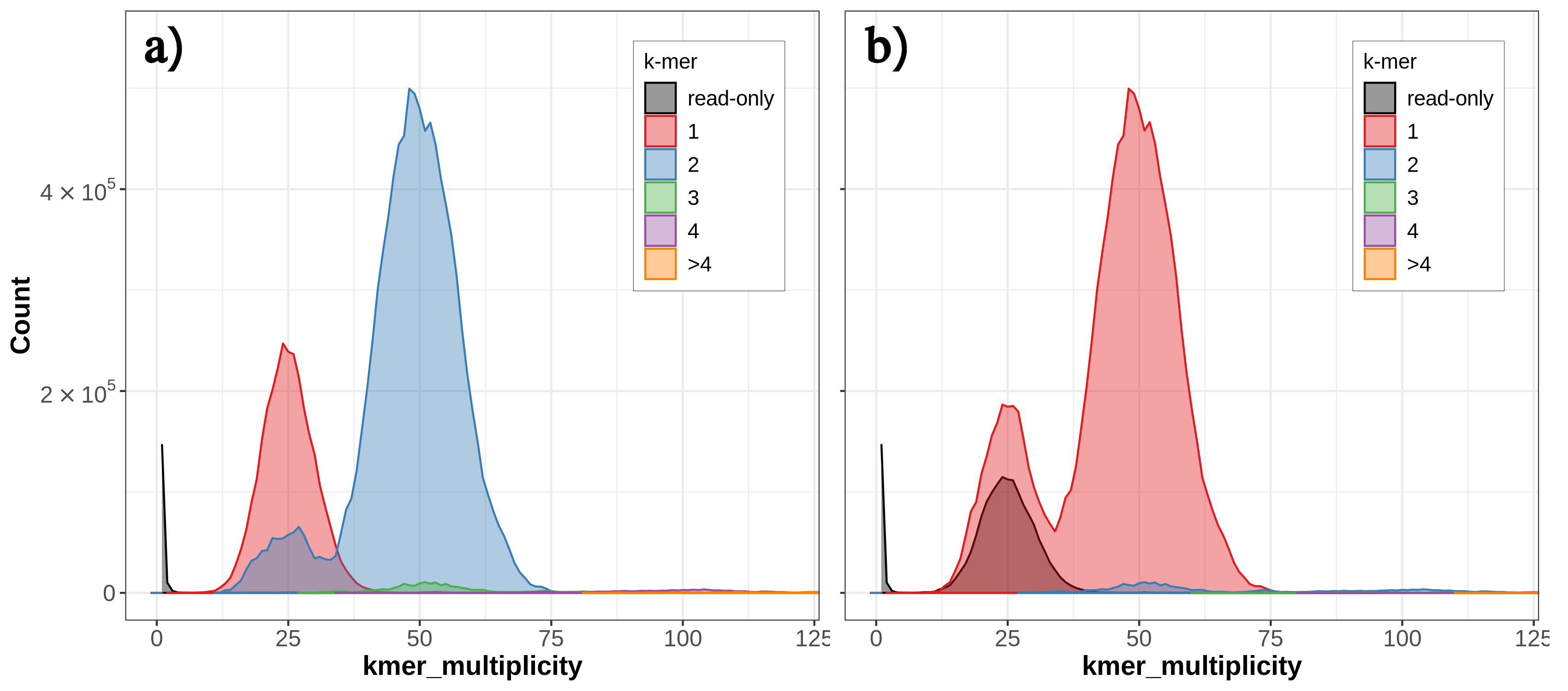
Thus, we know there is some false duplication (the 3-copy green bump) present as 2-copy in one of our assemblies, but we don’t know which one. We can look at the individual copy number spectrum for each haplotype in order to figure out which one contains the 2-copy k-mers (i.e., the false duplications). In the Merqury spectra-CN plot for hap2 we can see the small bump of 2-copy k-mers at around the 50 mark on the x-axis (fig. 6b).
Now that we know which haplotype contains the false duplications, we can run the purging workflow to try to get rid of these duplicates.
Purging with purge_dups
exchange Switch to step by step version
An ideal haploid representation would consist of one allelic copy of all heterozygous regions in the two haplotypes, as well as all hemizygous regions from both haplotypes (Guan et al. 2019). However, in highly heterozygous genomes, assembly algorithms are frequently not able to identify the highly divergent allelic sequences as belonging to the same region, resulting in the assembly of those regions as separate contigs. In order to prevent potential issues in downstream analysis, we are going to run the VGP purge assembly with purge_dups workflow, which will allow to identify and reassign heterozygous contigs. This step is only necessary if haplotypic duplications are observed, and the output should be carefully checked for overpurging.
Hands-on: VGP purge assembly with purge_dups pipeline workflow
- Click in the Workflow menu, located in the top bar
- Click in the workflow-run Run workflow buttom corresponding to
VGP purge assembly with purge_dups pipeline- In the Workflow: VGP purge assembly with purge_dups pipeline menu:
- param-file “Hifiasm Primary assembly”:
39: Hifiasm HiC hap1- param-file “Hifiasm Alternate assembly”:
40: Hifiasm HiC hap2- param-collection “Pacbio Reads Collection - Trimmed”:
22: Cutadapt- param-file “Genomescope model parameters”:
20: Genomescope on data 13 Model parameters- Click in the Run workflow buttom
This workflow generates a large number of outputs, among which we should highlight the datasets 74 and 91, which correspond to the purged primary and alternative assemblies respectively.
Hybrid scaffolding with Bionano optical maps
exchange Switch to step by step version
Once the assemblies generated by hifiasm have been purged, the next step is to run the VGP hybrid scaffolding with Bionano optical maps workflow. It will integrate the information provided by optical maps with primary assembly sequences in order to detect and correct chimeric joins and misoriented contigs. In addition, this workflow includes some additonal steps for evaluating the outputs.
Hands-on: VGP hybrid scaffolding with Bionano optical maps workflow
- Click in the Workflow menu, located in the top bar
- Click in the workflow-run Run workflow buttom corresponding to
VGP hybrid scaffolding with Bionano optical maps- In the Workflow: VGP hybrid scaffolding with Bionano optical maps menu:
- param-file “Bionano data”:
1: Bionano_dataset- param-file “Hifiasm Purged Assembly”:
90: Purge overlaps on data 88 and data 33: get_seqs purged sequences(note: the data numbers may differ in your workflow, but it should still be taggedp1from the purge_dups workflow)- param-file “Estimated genome size - Parameter File”:
60: Estimated Genome size- “Is genome large (>100Mb)?”:
No- Click on the Run workflow buttom
Once the workfow has finished, let’s have a look at the assembly reports.
As we can observe in the cumulative plot of the file 119 (fig. 7a), the total length of the assembly (12.160.926 bp) is slightly larger than the expected genome size. With respect to the NG50 statistic (fig. 7b), the value is 922.430 bp, which is significantly higher than the value obtained during the first evaluation stage (813.039 bp). This increase in NG50 means this scaffolded assembly is more contiguous compared to the non-scaffolded contigs.
It is also recommended to examine BUSCO outputs. In the summary image (fig. 7c), which can be found in the daset 117, we can appreciate that most of the universal single-copy orthologs are present in our assembly at the expected single-copy.
Question
- How many scaffolds are in the primary assembly after the hybrid scaffolding?
- What is the size of the largest scaffold? Has this changed with respect to the previous evaluation?
- What is the percentage of completeness on the core set genes in BUSCO? Has Bionano scaffolding increased the completeness?
- The number of contigs is 17.
- The largest contig is 1.531.728 bp long. This value hasn’t changed. This is expected, as the VGP pipeline implementation of Bionano scaffolding does not allow for breaking contigs.
- The percentage of complete BUSCOs is 95.7%. Yes, it has increased, since in the previous evaluation the completeness percentage was 88.7%.
Hi-C scaffolding
exchange Switch to step by step version
In this final stage, we will run the VGP hybrid scaffolding with HiC data, which exploits the fact that the contact frequency between a pair of loci strongly correlates with the one-dimensional distance between them. This information allows further scaffolding the Bionano scaffolds using SALSA2, usually generating chromosome-level scaffolds.
Hands-on: VGP hybrid scaffolding with HiC data
- Click in the Workflow menu, located in the top bar
- Click in the workflow-run Run workflow buttom corresponding to
VGP hybrid scaffolding with HiC data- In the Workflow: VGP hybrid scaffolding with HiC data menu:
- param-file “Scaffolded Assembly”:
114: Concatenate datasets on data 110 and data 109- param-file “HiC Forward reads”:
3: Hi-C_dataset_F (as fastqsanger)- param-file “HiC Reverse reads”:
2: Hi-C_dataset_R (as fastqsanger)- param-file “Estimated genome size - Parameter File”:
50: Estimated Genome size- “Is genome large (>100Mb)?”:
No- Click in the Run workflow buttom
In order to evaluate the Hi-C hybrid scaffolding, we are going to compare the contact maps before and after running the HiC hybrid scaffolding workflow (fig. 8), corresponding to the datasets 130 and 141 respectively.
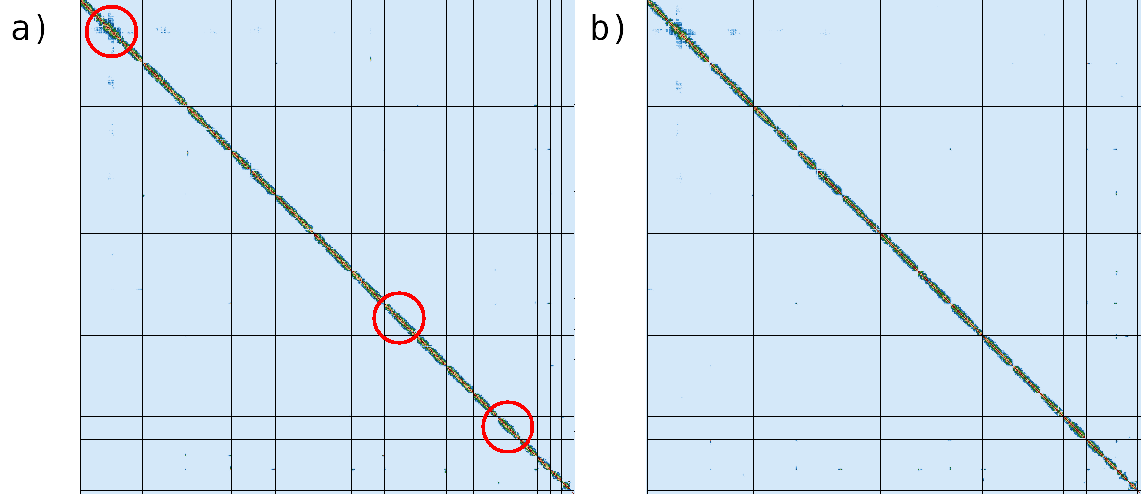
The regions marked with red circles highlight the most notable difference between the two contact maps, where inversion has been fixed.
Conclusion
To sum up, it is worthwhile to compare the final assembly with the S. cerevisiae S288C reference genome.
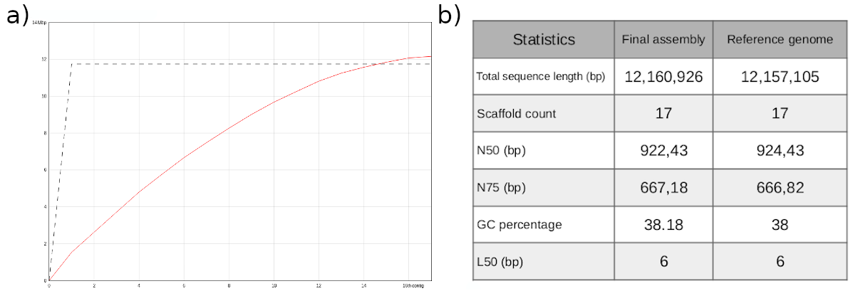
With respect to the total sequence length, we can conclude that the size of our genome assembly is almost identical to the reference genome (fig.9a,b). It is noteworthy that the reference genome consists of 17 sequences, while our assembly includes only 16 chromosomes. This is due to the fact that the reference genome also includes the sequence of the mitochondrial DNA, which consists of 85,779 bp. The remaining statistics exhibit very similar values (fig. 9b).
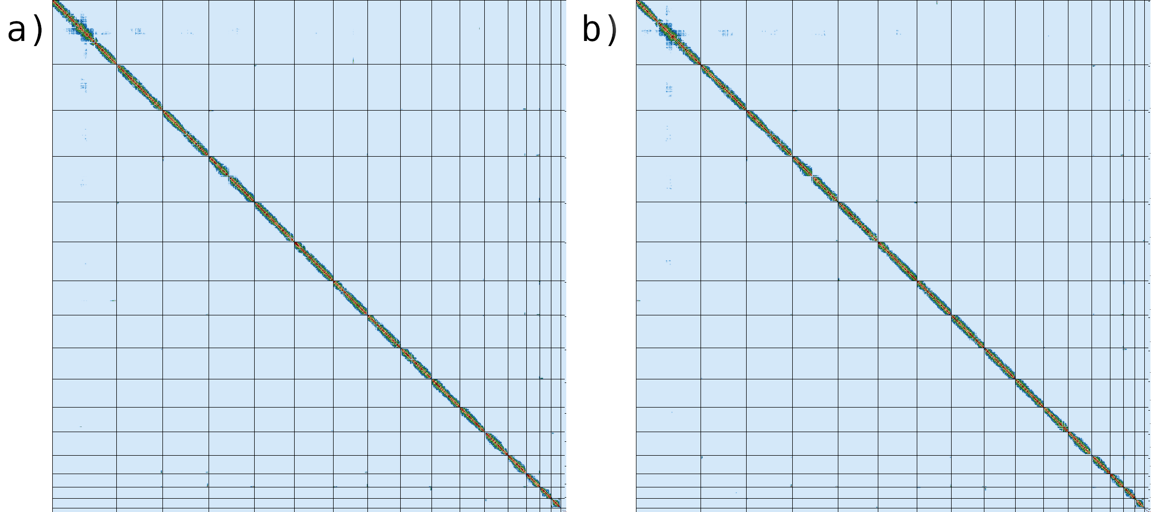
If we compare the contact map of our assembled genome (fig. 10a) with the reference assembly (fig. 10b), we can see that the two are indistinguishable, suggesting that we have generated a chromosome level genome assembly.
Key points
The VGP pipeline allows to generate error-free, near gapless reference-quality genome assemblies
The assembly can be divided in four main stages: genome profile analysis, HiFi long read phased assembly with hifiasm, Bionano hybrid scaffolding and Hi-C hybrid scaffolding
Frequently Asked Questions
Have questions about this tutorial? Check out the tutorial FAQ page or the FAQ page for the Assembly topic to see if your question is listed there. If not, please ask your question on the GTN Gitter Channel or the Galaxy Help ForumReferences
- Simão, F. A., R. M. Waterhouse, P. Ioannidis, E. V. Kriventseva, and E. M. Zdobnov, 2015 BUSCO: assessing genome assembly and annotation completeness with single-copy orthologs. Bioinformatics 31: 3210–3212. 10.1093/bioinformatics/btv351
- Guan, D., S. A. McCarthy, J. Wood, K. Howe, Y. Wang et al., 2019 Identifying and removing haplotypic duplication in primary genome assemblies. 10.1101/729962
- Rhie, A., B. P. Walenz, S. Koren, and A. M. Phillippy, 2020 Merqury: reference-free quality, completeness, and phasing assessment for genome assemblies. Genome Biology 21: 10.1186/s13059-020-02134-9
- Lariviere, D., A. Ostrovsky, C. Gallardo, A. Syme, L. Abueg et al., 2022 VGP assembly pipeline. Galaxy Training Network. https://training.galaxyproject.org/training-material/topics/assembly/tutorials/vgp_genome_assembly/tutorial.html#Rhie2021
Glossary
- G10K
- Genome 10K
- GWS
- Galaxy Workflow System
- Hi-C
- all-versus-all chromatin conformation capture
- HiFi
- high fidelity reads
- QV
- assembly consensus quality
- VGP
- Vertebrate Genome Project
- alternate assembly
- alternate loci not represented in the primary assembly
- contigs
- contiguous sequences in an assembly
- primary assembly
- homozygous regions of the genome plus one set of alleles for the heterozygous loci
- scaffolds
- one or more contigs joined by gap sequence
- unitig
Feedback
Did you use this material as an instructor? Feel free to give us feedback on how it went.
Did you use this material as a learner or student? Click the form below to leave feedback.
Citing this Tutorial
- Delphine Lariviere, Alex Ostrovsky, Cristóbal Gallardo, Brandon Pickett, Linelle Abueg, VGP assembly pipeline - short version (Galaxy Training Materials). http://0.0.0.0:4000/training-material/topics/assembly/tutorials/vgp_workflow_training/tutorial.html Online; accessed TODAY
- Batut et al., 2018 Community-Driven Data Analysis Training for Biology Cell Systems 10.1016/j.cels.2018.05.012
Congratulations on successfully completing this tutorial!@misc{assembly-vgp_workflow_training, author = "Delphine Lariviere and Alex Ostrovsky and Cristóbal Gallardo and Brandon Pickett and Linelle Abueg", title = "VGP assembly pipeline - short version (Galaxy Training Materials)", year = "", month = "", day = "" url = "\url{http://0.0.0.0:4000/training-material/topics/assembly/tutorials/vgp_workflow_training/tutorial.html}", note = "[Online; accessed TODAY]" } @article{Hiltemann_2023, doi = {10.1371/journal.pcbi.1010752}, url = {https://doi.org/10.1371%2Fjournal.pcbi.1010752}, year = 2023, month = {jan}, publisher = {Public Library of Science ({PLoS})}, volume = {19}, number = {1}, pages = {e1010752}, author = {Saskia Hiltemann and Helena Rasche and Simon Gladman and Hans-Rudolf Hotz and Delphine Larivi{\`{e}}re and Daniel Blankenberg and Pratik D. Jagtap and Thomas Wollmann and Anthony Bretaudeau and Nadia Gou{\'{e}} and Timothy J. Griffin and Coline Royaux and Yvan Le Bras and Subina Mehta and Anna Syme and Frederik Coppens and Bert Droesbeke and Nicola Soranzo and Wendi Bacon and Fotis Psomopoulos and Crist{\'{o}}bal Gallardo-Alba and John Davis and Melanie Christine Föll and Matthias Fahrner and Maria A. Doyle and Beatriz Serrano-Solano and Anne Claire Fouilloux and Peter van Heusden and Wolfgang Maier and Dave Clements and Florian Heyl and Björn Grüning and B{\'{e}}r{\'{e}}nice Batut and}, editor = {Francis Ouellette}, title = {Galaxy Training: A powerful framework for teaching!}, journal = {PLoS Comput Biol} Computational Biology} }
Galaxy Administrators: Install the missing toolsYou can use Ephemeris's
shed-tools installcommand to install the tools used in this tutorial.shed-tools install [-g GALAXY] [-a API_KEY] -t <(curl http://localhost:4000//training-material//api/topics/assembly/tutorials/vgp_workflow_training/tutorial.json | jq .admin_install_yaml -r)Alternatively you can copy and paste the following YAML
--- {}