OBIS is a global open-access data and information clearing-house on marine biodiversity for science, conservation and sustainable development. In order to visualize their marine data OBIS created the package obisindicators.
Obisindicators is an R library developed during the 2022 IOOS Code Sprint. The purpose was to create an ES50 diversity index within hexagonal grids following the diversity indicators notebook by Pieter Provoost linked above. The package includes several examples, limited to 1M occurrences, that demonstrate uses of the package.
This tutorial will guide you on getting obis marine data and processing them in order to calculate and visualize multiple indicators.
This tool for obisindicators is composed of 5 indicators : Number of record, Shannon, Simpson, Es50 and Hill which will be explained in more details later on.
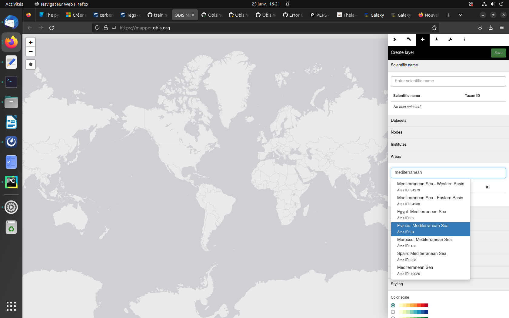
Go on the right panel and enter the criteria of your choise here in “Area” write down Mediterranean and select “France: Mediterranean Sea”.
Click on save on the top right
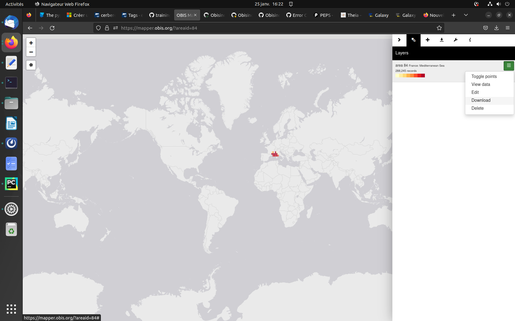
Figure 2: Obis download
Then on the 3 green lines top right press download
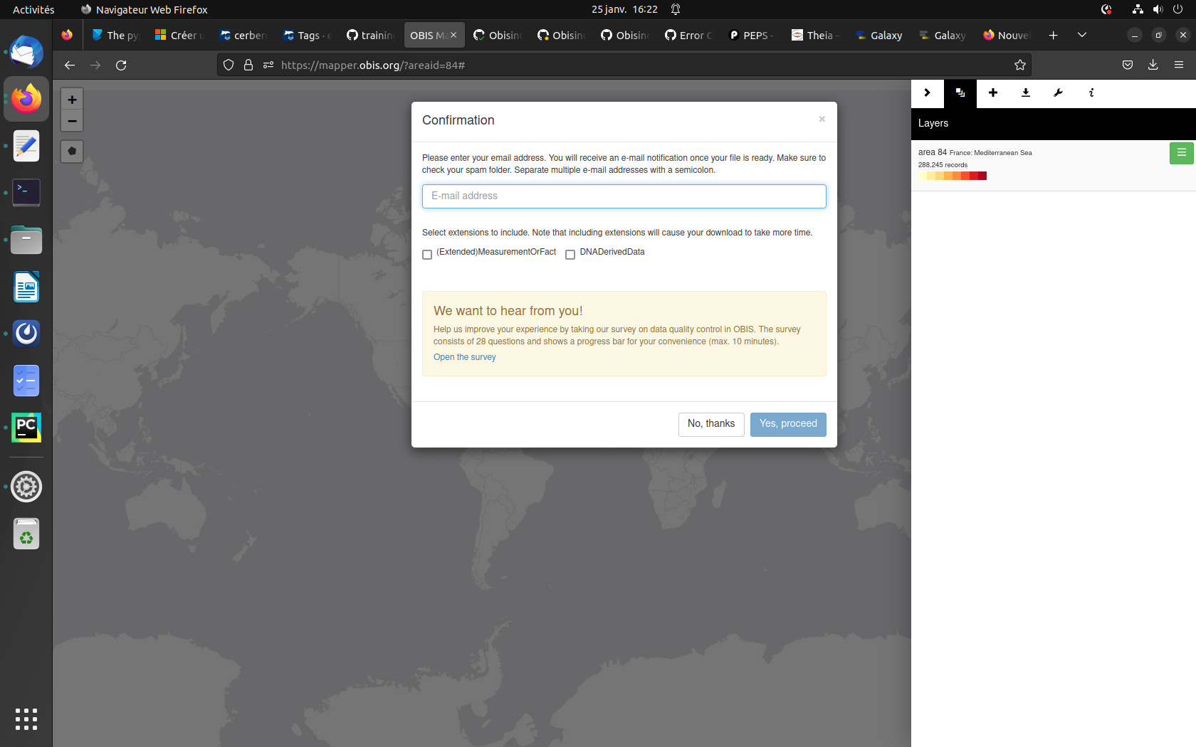
Enter your email on the pop-up screen and press Yes, procced
Figure 3: Waiting download
The download can take a while depending on the size of your dataset (here less than 15min)
Then click on Download ZIP file
Don’t forget to unzip your file on your machine.
In the downloaded folder you should have your data either csv format (Occurence.csv) and you must have at least 4 columns containing: latitude, longitude, species and record.
Upload obis data
Open the Galaxy Upload Manager galaxy-upload
Select Choose local files
Browse in your computer and get the downloaded zip folder
Press Start (it can take a few seconds to get ready)
Rename the datasets “obis data” for example and preview your dataset
Check the datatype must be csv or tabular
Click on the galaxy-pencilpencil icon for the dataset to edit its attributes
In the central panel, click on the galaxy-gearConvert tab on the top
In the lower part galaxy-chart-select-dataDatatypes, select datatypes
tip: you can start typing the datatype into the field to filter the dropdown menu
Click the Save button
Convert data csv-to-tabular
Hands-on: Convert your data
On your data in your history pannel click on param-text
In the top click on galaxy-gear Convert
Press exchange Create Dataset
Clean data Advanced Cut
Hands-on: Clean your data
Advanced CutTool: toolshed.g2.bx.psu.edu/repos/bgruening/text_processing/tp_cut_tool/1.1.0 with the following parameters:
“Cut by”: fields
“List of Fields”: c['1', '3', '4', '9', '95']
You are now all set to use your obis data in order to do a diversity analysis.
Ocean biodiversity indicators
Hands-on: Ocean biodiversity indicators
Ocean biodiversity indicatorsTool: toolshed.g2.bx.psu.edu/repos/ecology/obisindicators/obisindicators/0.0.1 with the following parameters:
“What character is the separator in your data? (Mostlikely a comma for a csv file and t for a tabular)”: Tabulator (\t)
“Select column containing the decimal value of the longitude “: c2
“Select column containing the decimal value of the latitude “: c3
“Select column containing the species “: c4
“Select column containing the number of records”: c5
“Type of projection for the map : select your coordinate reference system (CRS)”: Robinson Projection
“Choose a resolution for the discrete global grid”: 9
Note that you can rerun the tool and modify the resolution of the maps you want to create.
Click on Execute
You will see 5 outputs appear on the history pannel. one for each of the indicators
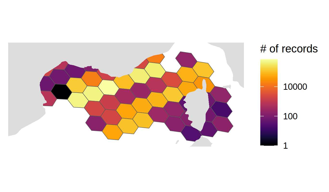
Number of records
Figure 4: Records map
In the table index the records correspond to n.
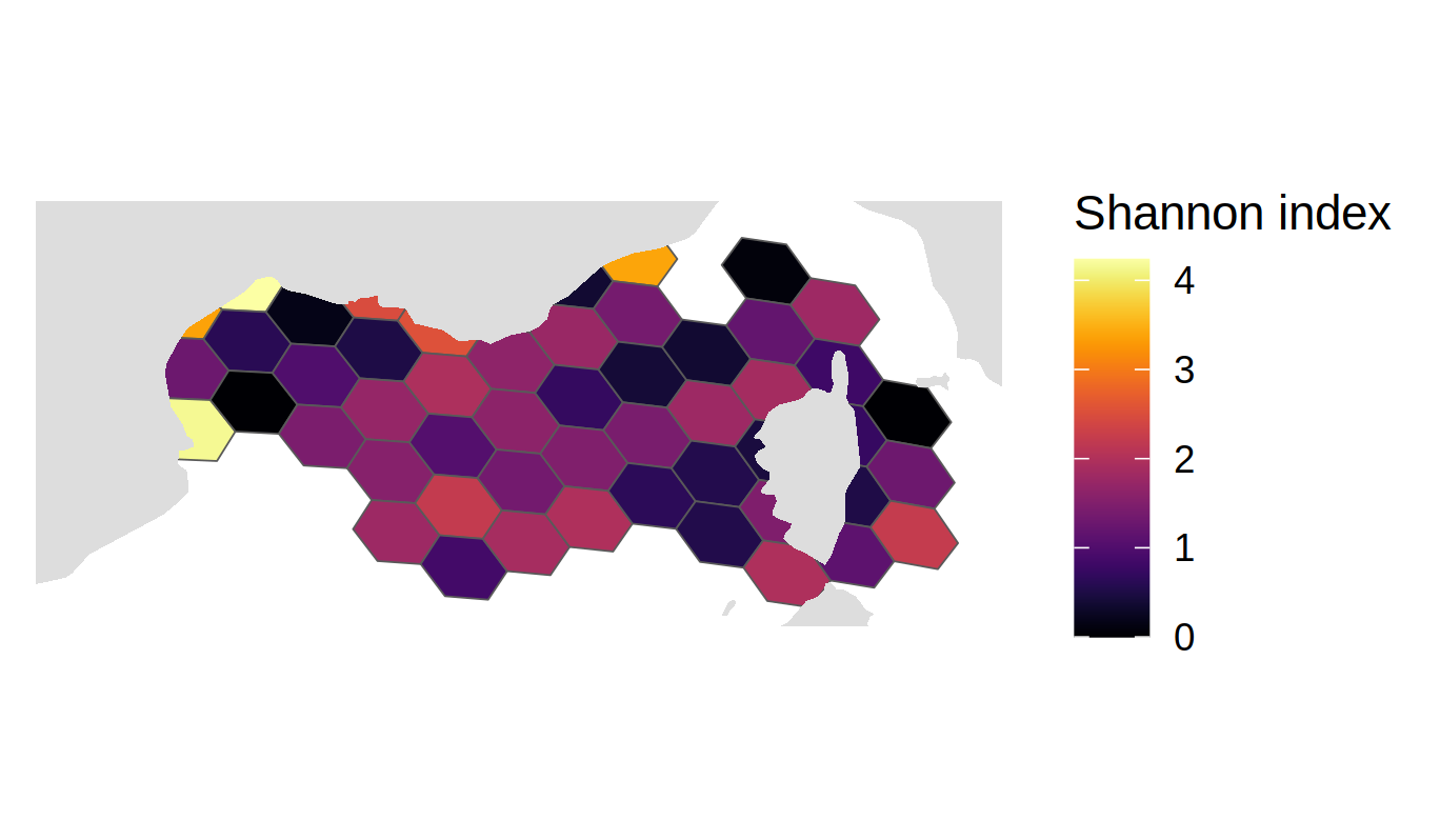
Shannon
The Shannon index expresses the uncertainty associated with the prediction of the species the next sampled individual belongs to. It assumes that individuals are randomly sampled from an infinitely large community, and that all species are represented in the sample.
Warning: OBIS uses records as a proxy for individuals and sampling is generally not random, the community is not infinitely large and not all species are represented in the sample.
The Shannon diversity index, also known as the Shannon-Wiener diversity index, is defined in OBIS as the sum over all species of $-fi*log(fi)$ with fi defined as $n/ni$ with n as the total number of records in the raster cell and ni as the total number of records for the ith-species in the raster cell.
Figure 5: Shannon map
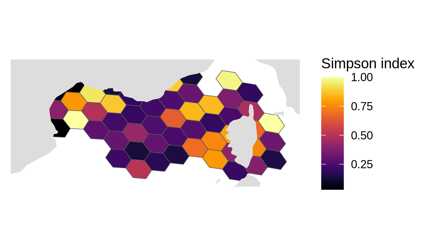
Simpson
The measure equals the probability that two entities taken at random from the dataset of interest represent the same type. It equals:
where is richness (the total number of types in the dataset) and is the proportional abundances of the types of interest.
Simpson’s index expresses the probability that any two individuals drawn at random from an infinitely large community belong to the same species. Note that small values are obtained in cells of high diversity and large values in cells of low diversity. This counterintuitive behavior is adressed with the Hill 2 number, which is the inverse of the Simpson index.
The Simpson biodiversity index is defined in OBIS as the sum over all species of $(ni/n)^2$ with n as the total number of records in the cell and ni the total number of records for the ith species.
Warning: The Simpson index has the same assumptions as the Shannon index.
Figure 6: Simpson map
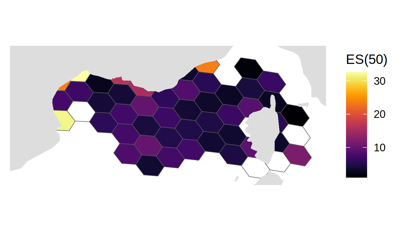
ES50
The expected number of marine species in a random sample of 50 individuals (records) is an indicator on marine biodiversity richness.
The ES50 is defined in OBIS as the $sum(esi)$ over all species of the following per species calculation:
when $n$ - ni$ $\ge$ $50$ (with n as the total number of records in the cell and ni the total number of records for the ith-species)
    $$ esi = 1 - exp(lngamma(n-ni+1) + lngamma(n-50+1) - lngamma(n-ni-50+1) - lngamma(n+1)) $$
when $n$ $\ge$ $50$
    $$ esi = 1 $$
else
    $$ esi = NULL $$
Warning: ES50 assumes that individuals are randomly distributed, the sample size is sufficiently large, the samples are taxonomically similar, and that all of the samples have been taken in the same manner.
Figure 7: ES50 map
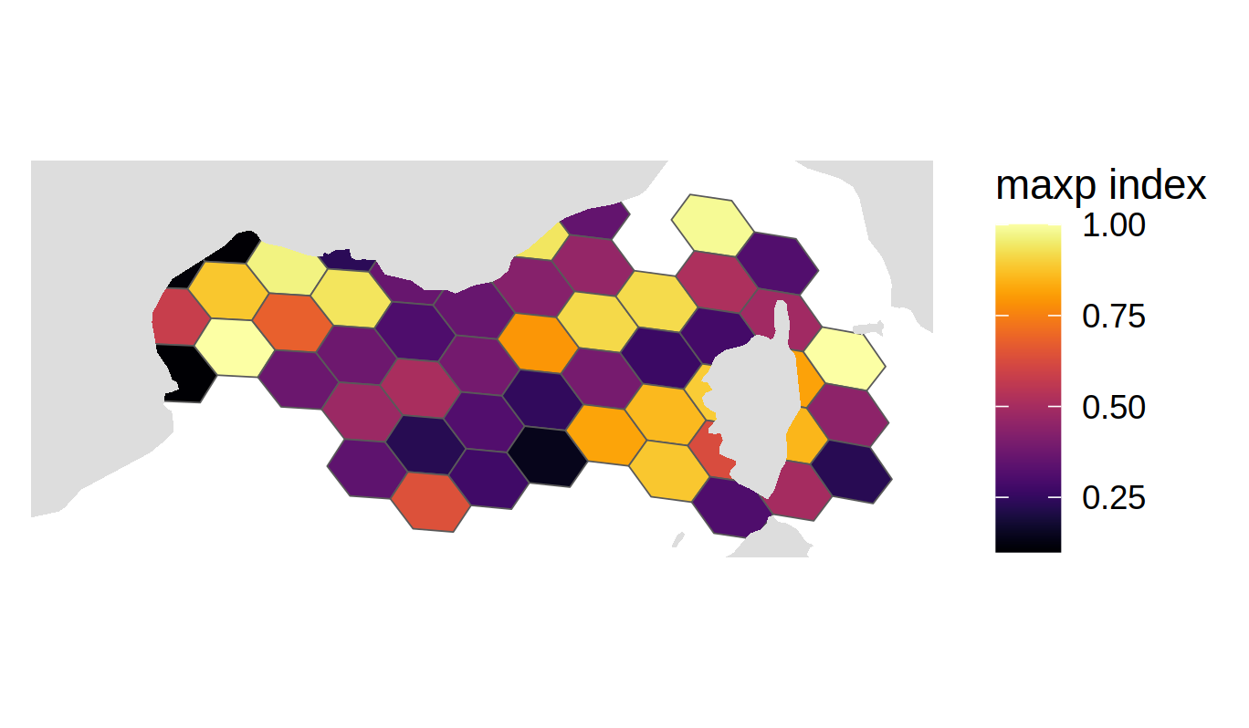
Maxp
Maxp is the maximum of the total number of records for the ith-species ni divided by the total number of records in the cell n, ie, \(Maxp = max(ni / n)\).
Figure 8: Maxp map
Hill
Hill 1
The Hill biodiversity index accounts for species’ relative abundance (number of records in OBIS) and Hill1 can be roughly interpreted as the number of species with “typical” abundances, and is a commonly used indicator for marine biodiversity richness. It is defined as:
Warning: The Simpson index has the same assumptions as the Shannon index.
Hill 2
The Hill biodiversity index accounts for species’ relative abundance (number of records in OBIS) and discounts rare species, so Hill2 can be interpreted as the equivalent to the number of more dominant species and so is less sensitive to sample size than Hill1. The Hill index is a commonly used indicator for marine biodiversity richness. It is defined as:
Warning: The Simpson index has the same assumptions as the Shannon index.
They are calculated as shown below:
- \(hill_1 = exp(shannon)\)
- \(hill_2 = 1 / simpson\)
- \(hill_inf = 1 / maxp\)
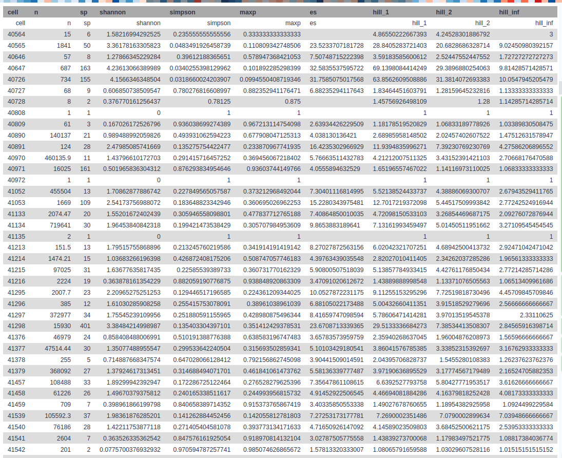
Index file
You also have a tabular file that sums up each indicators.
Figure 9: Tabular
Nb: the column sp is the count of the number of observations in a dataset. It is the number of records in the dataset.
Conclusion
You here learn how to select and download OBIS dataset for your region of interest, to handle data to finally compute diversity indicators and display it in maps.
Further information, including links to documentation and original publications, regarding the tools, analysis techniques and the interpretation of results described in this tutorial can be found here.
Feedback
Did you use this material as an instructor? Feel free to give us feedback on how it went.
Did you use this material as a learner or student? Click the form below to leave feedback.
Batut et al., 2018 Community-Driven Data Analysis Training for Biology Cell Systems 10.1016/j.cels.2018.05.012
@misc{ecology-obisindicators,
author = "Marie Josse and Yvan Le Bras",
title = "Obis marine indicators (Galaxy Training Materials)",
year = "",
month = "",
day = ""
url = "\url{http://0.0.0.0:4000/training-material/topics/ecology/tutorials/obisindicators/tutorial.html}",
note = "[Online; accessed TODAY]"
}
@article{Hiltemann_2023,
	doi = {10.1371/journal.pcbi.1010752},
	url = {https://doi.org/10.1371%2Fjournal.pcbi.1010752},
	year = 2023,
	month = {jan},
	publisher = {Public Library of Science ({PLoS})},
	volume = {19},
	number = {1},
	pages = {e1010752},
	author = {Saskia Hiltemann and Helena Rasche and Simon Gladman and Hans-Rudolf Hotz and Delphine Larivi{\`{e}}re and Daniel Blankenberg and Pratik D. Jagtap and Thomas Wollmann and Anthony Bretaudeau and Nadia Gou{\'{e}} and Timothy J. Griffin and Coline Royaux and Yvan Le Bras and Subina Mehta and Anna Syme and Frederik Coppens and Bert Droesbeke and Nicola Soranzo and Wendi Bacon and Fotis Psomopoulos and Crist{\'{o}}bal Gallardo-Alba and John Davis and Melanie Christine Föll and Matthias Fahrner and Maria A. Doyle and Beatriz Serrano-Solano and Anne Claire Fouilloux and Peter van Heusden and Wolfgang Maier and Dave Clements and Florian Heyl and Björn Grüning and B{\'{e}}r{\'{e}}nice Batut and},
	editor = {Francis Ouellette},
	title = {Galaxy Training: A powerful framework for teaching!},
	journal = {PLoS Comput Biol} Computational Biology}
}
Funding
These individuals or organisations provided funding support for the development of this resource
This project (2020-1-NL01-KA203-064717) is funded with the support of the Erasmus+ programme of the European Union. Their funding has supported a large number of tutorials within the GTN across a wide array of topics.
Congratulations on successfully completing this tutorial!
Galaxy Administrators: Install the missing tools
You can use Ephemeris's shed-tools install command to install the tools used in this tutorial.
 Marie Josse
 Yvan Le Bras
Questions: