Discovered over 40 years ago, alternative splicing (AS) formed a large part of the puzzle explaining how proteomic complexity can be achieved with a limited set of genes (Alt 1980). The majority of eukaryote genes have multiple transcriptional isoforms, and recent data indicate that each transcript of protein-coding genes contain 11 exons and produce 5.4 mRNAs on average (Piovesan et al. 2016). In humans, approximately 95% of multi-exon genes show evidence of AS and approximately 60% of genes have at least one alternative transcription start site, some of which exert antagonistic functions (Carninci et al. 2006, Miura et al. 2012). Its regulation is essential for providing cells and tissues their specific features, and for their response to environmental changes (Wang et al. 2008, Kalsotra and Cooper 2011).
Alterations in gene splicing has been demonstrated to have significant impact on cancer development, and multiple evidences indicate that its disruption can exhibit effects on virtually all aspect of tumor progression (Namba et al. 2021, Bonnal et al. 2020). For instance, the unannotated isoform of TNS3 was found to be a novel driver of breast cancer (Namba et al. 2021).
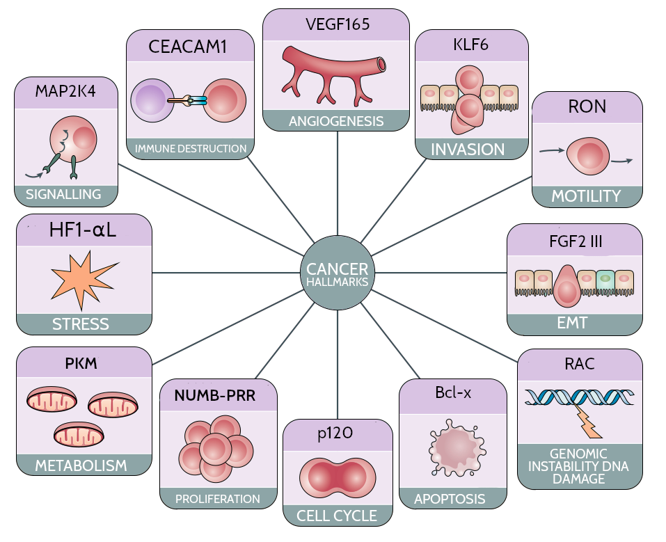
Figure 1: Effect of alternative splicing dysregulation on cancer progression. The diagram depicts various cancer hallmarks and examples of genes whose splicing dysregulation has been demostrated to be implicated in the corresponding functional modification.
Disregulation in AS can lead to the activation of oncogenes (OCGs) or the inactivation of tumor supression genes (TSGs), which can promote or suppress tumorigenesis, respectively (Bashyam et al. 2019). However, the strict classification of cancer genes as either OCGs or TSGs may be an oversimplification, as some genes can exhibit a dual role in cancer development, often impacting the same facet of tumorigenesis (Bashyam et al. 2019). One of the mechanism that has been proposed to partially explain this apparently contradictory effect is the differential usage of isoforms, often referred to as isoform switching (IS). This regulatory phenomenon has been demonstrated to have a substantial biological impact in a diverse range of biological contexts, caused by functional diversity potential of the different isoforms (Vitting-Seerup and Sandelin 2017).
In this tutorial, we aim to perform a genome-wide analysis of IS in cancer, with the objective of identifying genes of potential clinical relevance and gene regulatory networks on genome-scale.
The datasets consist of twelve FASTQ files, generated through the Illumina NovaSeq 6000 sequencing system. Half of the samples were obtained from PANC1 tumour lines, and the rest from control cells. The protocol used for extracting the samples includes the depletion of rRNAs by subtractive hybridization, a general strategy for mRNA enrichment in RNA-seq samples. For this training we will use a reduced set of reads, in order to speed up the analysis. The original datasets are available in the NCBI SRA database, with the accession number PRJNA542693.
Get data
The first step of our analysis consists of retrieving the RNA-seq datasets from Zenodo and organizing them into collections.
Hands-on: Retrieve miRNA-Seq and mRNA-Seq datasets
Create a new history for this tutorial
Import the files from Zenodo:
Open the file galaxy-uploadupload menu
Click on Rule-based tab
“Upload data as”: Collection(s)
Copy the following tabular data, paste it into the textbox and press Build
From Rules menu select Add / Modify Column Definitions
Click Add Definition button and select List Identifier(s): column A
Then you’ve chosen to upload as a ‘dataset’ and not a ‘collection’. Close the upload menu, and restart the process, making sure you check Upload data as: Collection(s)
Click Add Definition button and select URL: column B
Click Add Definition button and select Type: column C
Click Add Definition button and select Pair-end Indicator: column D
Click Apply, give a name to your collection like All samples and press Upload
Next we will retrieve the remaining datasets.
Hands-on: Retrieve the additional datasets
Import the files from Zenodo:
Open the file galaxy-uploadupload menu
Click on Rule-based tab
“Upload data as”: Datasets
Once again, copy the tabular data, paste it into the textbox and press Build
From Rules menu select Add / Modify Column Definitions
Click Add Definition button and select Name: column A
Click Add Definition button and select URL: column B
Click Apply and press Upload
As indicated above, for this tutorial the depth of the samples was reduced in order to speed up the time needed to carry out the analysis. This was done as follows:
Hands-on: Dataset subsampling
Convert FASTA to TabularTool: CONVERTER_fasta_to_tabular converter with the following parameters:
param-files“Fasta file”: GRCh38.p13.genome.fa.gz
Search in textfilesTool: toolshed.g2.bx.psu.edu/repos/bgruening/text_processing/tp_grep_tool/1.1.1 converter with the following parameters:
param-files“Select lines from”: Output of Convert FASTA to Tabular
“Regular Expression2”: chr5
Tabular-to-FASTATool: toolshed.g2.bx.psu.edu/repos/devteam/tabular_to_fasta/tab2fasta/1.1.1 converter with the following parameters:
param-files“Tab-delimited file”: Output of Search in textfiles
“Title column(s)”: Column: 1
“Sequence column”: Column: 2
HISAT2Tool: toolshed.g2.bx.psu.edu/repos/iuc/hisat2/hisat2/2.2.1+galaxy1 converter with the following parameters:
In “Source for the reference genome”: Use a genome from history
param-files“Select the reference genome”: Output of Tabular-to-FASTA
In “Is this a single or paired library”: Paired-end Dataset Collection
“Paired Collection”: Select the collection of the original datasets
In “Output options”: Specify output options
“Write aligned reads (in fastq format) to separate file(s)”: Yes
It will generate three collections: one with the aligned BAM files, one with the FASTQ files corresponding with the forward reads, and one with the FASTQ files corresponding to the reverse reads. Those FASTQ files are the ones that will be used in this training.
Quality assessment
Once we have got the datasets, we can start with the analysis. The first step is to perform the quality assessment. Since this step is deeply covered in the tutorial Quality control, we won’t describe this section in detail.
Comment: Initial quality evaluation (OPTIONAL)
For the initial quality evaluation, it is necessary to perform a pre-processing step consisting in flattening the list of pairs into a simple list; this step is required because of issues between FastQC and MultiQC. The Raw data QC files generated by FastQC will be combine into a a single one by making use of MultiQC.
Hands-on: Initial quality evaluation
Flatten collectionTool: FLATTEN with the following parameters convert the list of pairs into a simple list:
“Input Collection”: All samples
FastQCTool: toolshed.g2.bx.psu.edu/repos/devteam/fastqc/fastqc/0.73+galaxy0 with the following parameters:
param-collection“Raw read data from your current history”: Output of Flatten collectiontool selected as Dataset collection
Click on param-collectionDataset collection in front of the input parameter you want to supply the collection to.
Select the collection you want to use from the list
MultiQCTool: toolshed.g2.bx.psu.edu/repos/iuc/multiqc/multiqc/1.11+galaxy1 with the following parameters:
In “Results”:
param-repeat“Insert Results”
“Which tool was used generate logs?”: FastQC
In “FastQC output”:
param-repeat“Insert FastQC output”
param-collection“FastQC output”: FastQC on collection: Raw data (output of FastQCtool)
“Report title”: Raw data QC
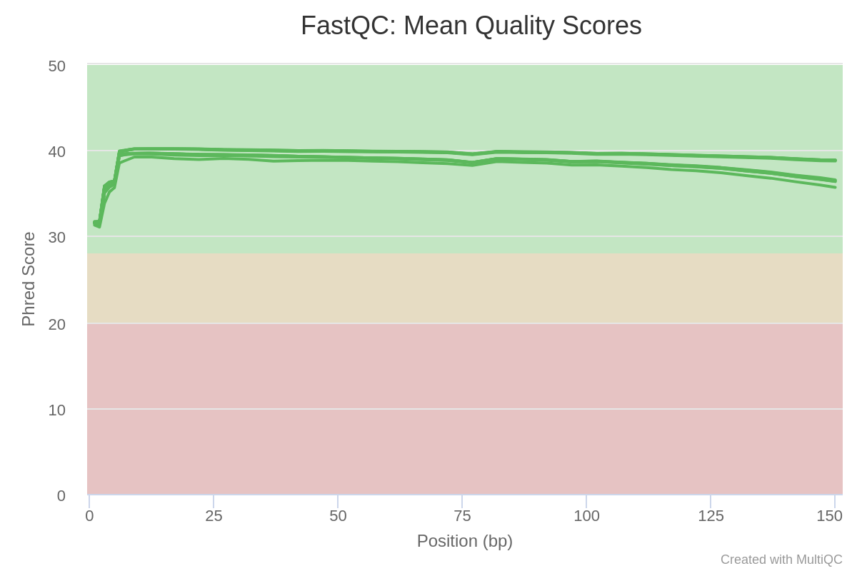
Let’s evaluate the per base sequence quality and the adapter content.
Figure 2: MultiQC aggregated reports. Mean quality scores.
As we can appreciate in the figure the per base quality of all reads seems to be very good, with values over 30 in all cases. In addition, according the report no samples werefound with adapter contamination higher than 0.1%.
Read pre-processing with fastp
In order to remove the adaptors we will make use of fastp, which is able to detect the adapter sequence by performing a per-read overlap analysis, so we won’t even need to specify the adapter sequences.
Hands-on: Pre-process reads with fastp
fastpTool: toolshed.g2.bx.psu.edu/repos/iuc/fastp/fastp/0.23.2+galaxy0 with the following parameters:
“Single-end or paired reads”: Paired Collection
param-collection“Select paired collection(s)”: All samples
In “Global trimming options”:
“Trim front for input 1”: 10
In “Overrepresented Sequence Analysis”:
“Enable overrepresented analysis”: Yes
“Overrepresentation sampling”: 50
In “Filter Options”:
In “Quality filtering options”:
“Qualified quality phred”: 20
Rename the output fastp on collection X: Paired-end output as Trimmed samples
RNA-seq mapping and isoform quantification
The following section can be considered as the hard-core part of the training, the reason is not because of it’s complexity (not all the details about the computational procedures will be presented, just those elements required for a basic understanding), but because it allows to characterize isoform quantification approach as genome-guided-based method.
Comment: Transcriptome-reconstruction approaches
The different methods for estimating transcript/isoform abundance can be classified depending on two main requirements: reference sequence and alignment. Reference-guided transcriptome assembly strategy requires to aligning sequencing reads to a reference genome first, and then assembling overlapping alignments into transcripts. In contrast, de novo transcriptome assembly methods directly reconstructs overlapping reads into transcripts by utilising the redundancy of sequencing reads themselves (Lu et al. 2013).
In that section makes use of three main tools: RNA STAR, considered a state-of-the-art mapping tool for RNA-seq data, RSeQC, a package that allows comprehensively evaluate different aspects of the RNA-seq data, and StringTie, which uses a genome-guided transcriptome assembly approach along with concepts from de novo genome assembly to perform transcript assembly and quantification.
RNA-seq mapping with RNA STAR
RNA STAR is a splice-aware RNA-seq alignment tool that allows to identify canonical and non-canonical splice junctions by making use of sequential maximum mappable seed search in uncompressed suffix arrays followed by seed clustering and stitching procedure (Križanović et al. 2017). One advantage of RNA STAR with respect to other tools is that it includes a feature called two-pass mode, a framework in which splice junctions are separately discovered and quantified, allowing robustly and accurately identify splice junction patterns for differential splicing analysis and variant discovery.
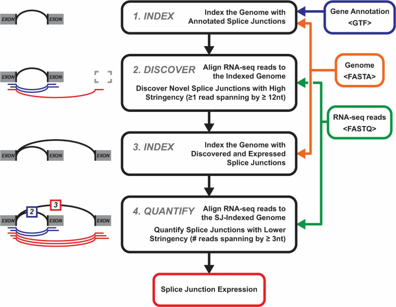
During two-pass mode splice junctions are discovered in a first alignment pass with high stringency, and are used as annotation in a second pass to permit lower stringency alignment, and therefore higher sensitivity (fig. 3). Two-pass alignment enables sequence reads to span novel splice junctions by fewer nucleotides, conferring greater read depth and providing significantly more accurate quantification of novel splice junctions that one-pass alignment (Veeneman et al. 2015).
Figure 3: Two-pass alignment flowchart. Center and right, stepwise progression of two-pass alignment. First, the genome is indexed with gene annotation. Next, novel splice junctions are discovered from RNA sequencing data at a relatively high stringency (12 nt minimum spanning length). Third, these discovered splice junctions, and expressed annotated splice junctions are used to re-index the genome. Finally, alignment is performed a second time, quantifying novel and annotated splice junctions using the same, relatively lower stringency (3 nt minimum spanning length), producing splice junction expression. Source: Veeneman et al., 2016.
The choice of RNA STAR as mapper is also determined by the sequencing technology; it has been demonstrated adequate for short-read sequencing data, but when using long-read data, such as PacBio or ONT reads, it is recommended to use GMAP as alignment tool (Križanović et al. 2017).
Comment: Intron spanning in RNA-seq analysis
RNA-seq mappers need to face the challenge associated with intron spanning of mature mRNA molecules, from which introns have been removed by splicing (single short read might align to two locations that are separated by 10 kbp or more). The complexity of this operation can be better understood if we take in account that for a typical human RNA-seq data set using 100-bp reads, more than 35% of the reads will span multiple exons.
So, let’s perform the mapping step.
Hands-on: Task description
RNA STARTool: toolshed.g2.bx.psu.edu/repos/iuc/rgrnastar/rna_star/2.7.10b+galaxy3 with the following parameters:
“Single-end or paired-end reads”: Paired-end (as collection)
param-collection“RNA-Seq FASTQ/FASTA paired reads”: Trimmed samples (output of fastptool)
“Custom or built-in reference genome”: Use reference genome from history and create temporary index
param-file“Select a reference genome”: GRCh38.p13.genome.fa.gz
“Build index with or without known splice junctions annotation”: build index with gene-model
param-file“Gene model (gff3,gtf) file for splice junctions”: gencode.v43.annotation.gtf.gz
“Use 2-pass mapping for more sensitive novel splice junction discovery”: Yes, perform single-sample 2-pass mapping of all reads
“Compute coverage”: Yes in bedgraph format
“Generate a coverage for each strand (stranded coverage)”: No
Rename the output RNA STAR on collection X: mapped.bam as Mapped collection
Before moving to the transcriptome assembly and quantification step, we are going to use RSeQC in order to obtain some RNA-seq-specific quality control metrics.
RNA-seq specific quality control metrics with RSeQC
RNA-seq-specific quality control metrics, such as sequencing depth, read distribution and coverage uniformity, are essential to ensure that the RNA-seq data are adequate for transcriptome reconstruction and AS analysis. For example, the use of RNA-seq with unsaturated sequencing depth gives imprecise estimations and fails to detect low abundance splice junctions, limiting the precision of many analyses (Wang et al. 2012).
In this section we will make use of of the RSeQC toolkit in order to generate the RNA-seq-specific quality control metrics. But before starting, we need to convert the annotation GTF file into BED12 format, which will be required in subsequent steps.
Hands-on: GTF to BED12 GTF conversion
Convert GTF to BED12Tool: toolshed.g2.bx.psu.edu/repos/iuc/gtftobed12/gtftobed12/357 with the following parameters:
param-file“GTF File to convert”: gencode.v43.annotation.gtf.gz
“Advanced options”: Set advanced options
“Ignore groups without exons”: Yes
Rename the output as BED12 annotation
We are going to use the following RSeQC modules:
Infer Experiment: inference of RNA-seq configuration
Gene Body Coverage: compute read coverage over gene bodies
Junction Saturation: check junction saturation
Junction Annotation: compares detected splice junctions to a reference gene model
Read Distribution: calculates how mapped reads are distributed over genome features
Once all required outputs have been generated, we will integrate them by using MultiQC in order to interpret the results.
Hands-on: Raw reads QC
Infer ExperimentTool: toolshed.g2.bx.psu.edu/repos/nilesh/rseqc/rseqc_infer_experiment/5.0.1+galaxy1 with the following parameters:
param-collection“RSeQC gene body coverage: stats file”: select stats (TXT) collections
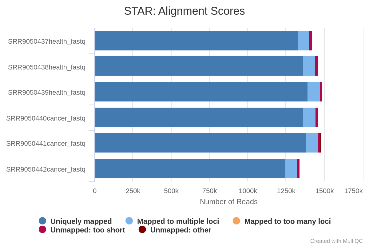
First, we will evaluate the plot corresponding to the RNA STAR alignment scores (fig. 4), which will allow us to easily compare the samples to get an overview of the quality of the samples. As a general criteria, we can consider that good quality samples should have at least 75% of the reads uniquely mapped. In our case, of samples have unique mapping values over 90%.
Figure 4: RNA star alignment stats plot. Note that STAR counts a paired-end read as one read.
Now we can have a look at the RSeQC results; we will evaluate the RSeQC Read Distribution plot (fig. 5).
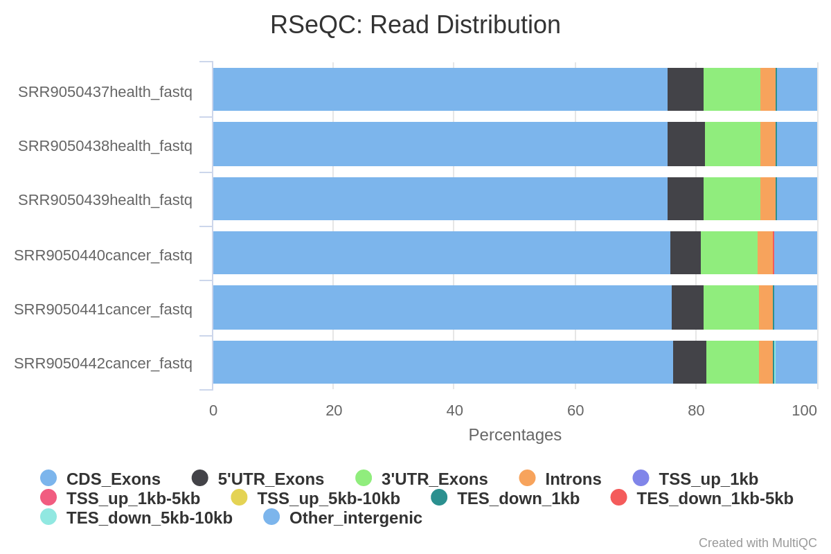
Figure 5: RSeQC read distribution. This module will calculate how mapped reads were distributed over genome feature (like CDS exon, 5’UTR exon, 3’ UTR exon, Intron, Intergenic regions).
In that case, all samples show a similar trend, both in health and cancer samples, with most reads mapping on CDS exons (around 72%), 5’UTR (around 4.5%) and 3’UTR (around 13.5%).
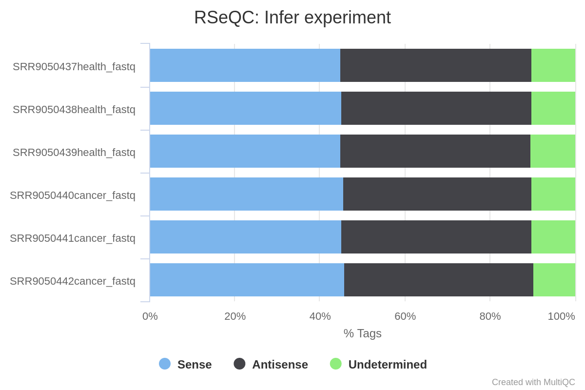
Now we will evaluate the results of the Infer Experiment module, which allows to speculate the experimental design (whether sequencing is strand-specific, and if so, how reads are stranded) by sampling a subset of reads from the BAM file and comparing their genome coordinates and strands with those of the reference gene model (Wang et al. 2012).
Figure 6: RSeQC Infer Experiment plot. It counts the percentage of reads and read pairs that match the strandedness of overlapping transcripts. It can be used to infer whether RNA-seq library preps are stranded (sense or antisense).
As can be appreciated in the image, the proportion of reads assigned as sense is similar to the ones assigned as antisense, which indicates that in that case our RNA-seq data is non-strand specific.
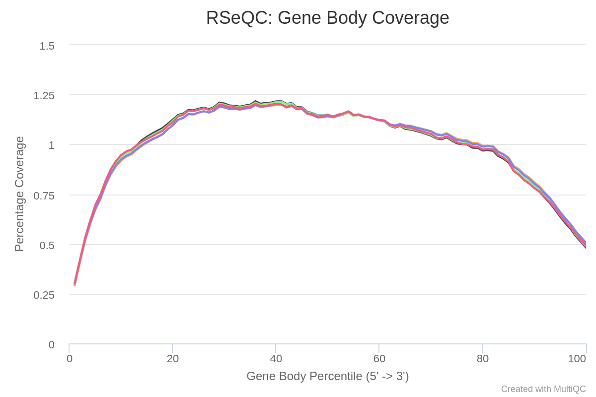
Now, let’s evaluate the results generated by the Gene Body Coverage module. It scales all transcripts to 100 nt and calculates the number of reads covering each nucleotide position. The plot generated from this information illustrates the coverage profile along the gene body, defined as the entire gene from the transcription start site to the end of the transcript (fig. 7).
Figure 7: RSeQC gene body coverage plot. It calculates read coverage over gene bodies. This is used to check if reads coverage is uniform and if there is any 5' or 3' bias.
The gene body coverage pattern is highly influenced by the RNA-seq protocol, and it is useful for identifying artifacts such as 3’ skew in libraries. For example, a skew towards increased 3’ coverage can happen in degraded samples prepared with poly-A selection. According the figure 5, there’re not bias in our reads as a result of sequencing technical problems.
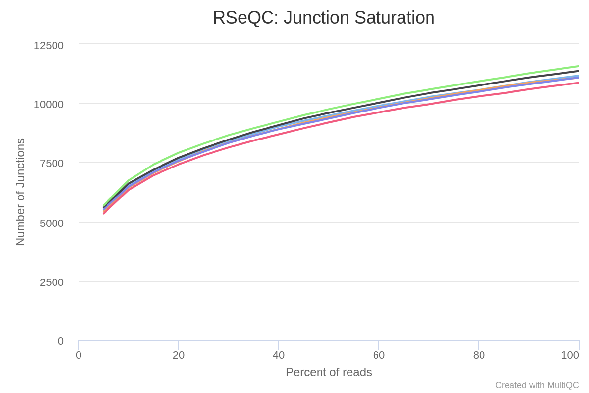
Other important metric for AS analysis is the one provided by the Junction Saturation module, which allows to determine if the current sequencing depth is sufficient to perform AS analyses by comparing the detected splice junctions to reference gene model (fig. 8).
Since for a well annotated organism both the number of expressed genes and spliced junctions is considered to be almost fixed, if the number of known junctions reaches a plateau means that the current sequencing depth is almost saturated for known junction detection. In other words, nearly all known junctions have already been detected, and deeper sequencing will not likely detect additional known junctions. Using an unsaturated sequencing depth would miss many rare splice junctions (Wang et al. 2012).
Comment: RSeQC junction saturation details
This approach helps identify if the sequencing depth is sufficient for AS analysis. However, it relies on the reference gene model for junction comparison, which might not be complete or accurate for all organisms. In addition, it might not provide enough information for novel junction detection, as the sequencing depth might still be insufficient for detecting new splice junctions.
Figure 8: RSeQC junction saturation. Saturation is checked by re-sampling the alignments from the BAM file, and the splice junctions from each subset is detected (green) and and compared them to the reference model (grey).
As we can appreciate in the plot, the known junctions tend to stabilize around 110.000, which indicates that the read sequencing depth is good enough for performing the AS analysis.
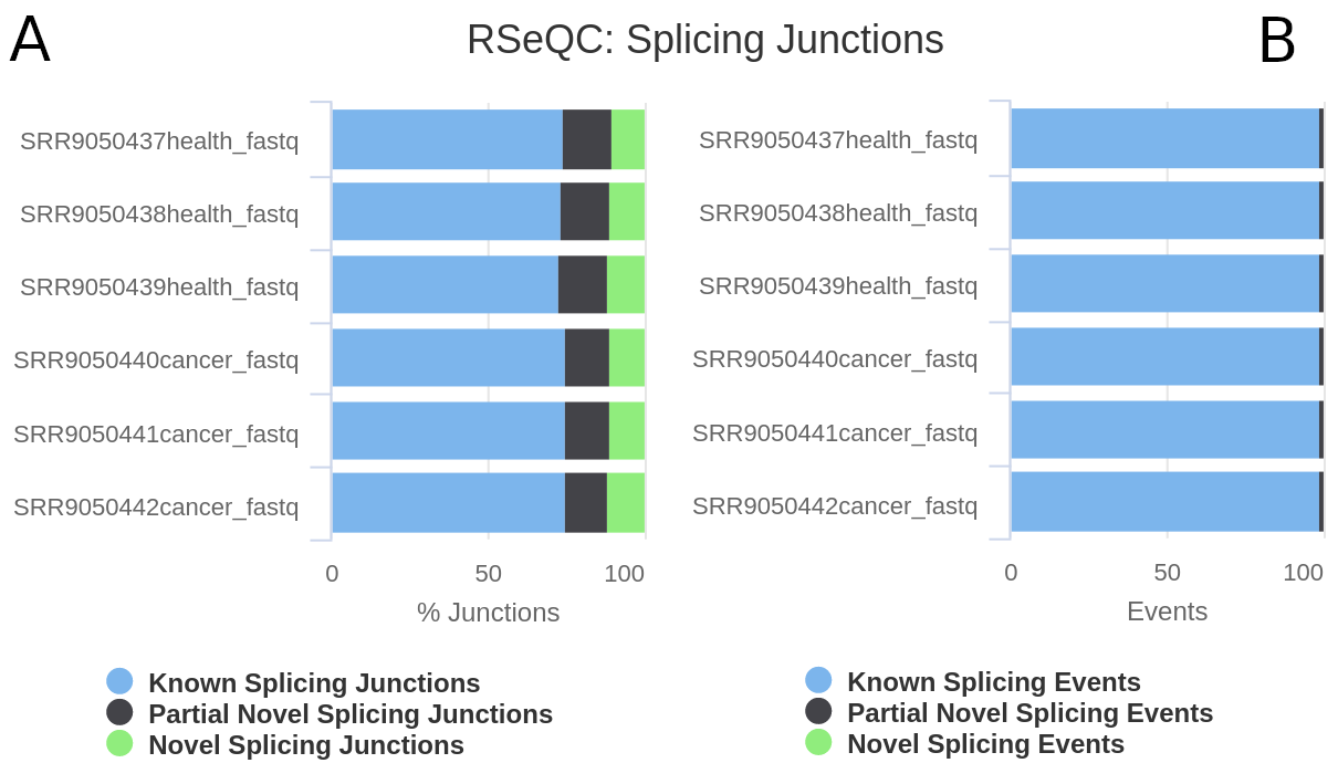
After confirming that the saturation level is good enough, finally, we will check the output generated by the RSeQC junction annotation module; it allows to evaluate both splice junctions (multiple reads show the same splicing event) and splice events (single read level) (fig. 9).
Figure 9: RSeQC junction annotation. The detected junctions and events are divided in three exclusive categories: known splicing junctions (blue), partial novel splicing junction (one of the splice site is novel) (grey) and new splicing junctions (green). Splice events refer to the number of times a RNA-read is spliced (A). Splice junctions correspond to multiple splicing events spanning the same intron.
According to the results, despite the number of new (or partially new) splicing junctions is relatively slow (around 0.5%), a large proportion of reads show novel splicing junction patterns.
After evaluating the quality of the RNA-seq data, we can start with the transcriptome assembly step.
Transcriptome assembly and quantification with StringTie
StringTie is a fast and highly efficient assembler of RNA-seq alignments into potential transcripts. It uses a network flow algorithm to reconstruct transcripts and quantitate them simultaneously. This algorithm is combined with an assembly method to merge read pairs into full fragments in the initial phase (Kovaka et al. 2019, Pertea et al. 2015).
Comment: StringTie algorithm
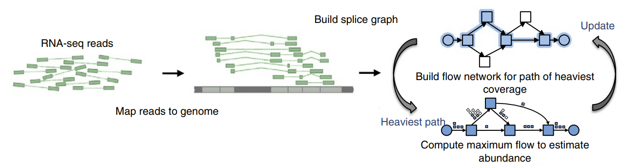
StringTie first groups the reads into clusters, collapsing the reads that align to the identical location on the genome and keeping a count of how many alignments were collapsed, then creates a splice graph for each cluster from which it identifies transcripts, and then for each transcript it creates a separate flow network to estimate its expression level using a maximum flow algorithm (Pertea et al. 2015) (fig. 10).
Figure 10: Transcript assembly pipeline for StringTie. It begins with a set of RNA-seq reads that have been mapped to the genome. StringTie iteratively extracts the heaviest path from a splice graph, constructs a flow network, computes maximum flow to estimate abundance, and then updates the splice graph by removing reads that were assigned by the flow algorithm. This process repeats until all reads have been assigned. Source: Perea et al., 2015
StringTie uses an aggressive strategy for identifying and removing spurious spliced alignments. If a spliced read is aligned with more than 1% mismatches, keeping in mind that Illumina sequencers have an error rate < 0.5%, then StringTie requires 25% more reads than usual (the default is 1 read per bp) to support that particular spliced alignment. In addition, if a spliced read spans a very long intron (more than 100,000 bp), StringTie accepts that alignment (and the intron) only if a larger anchor of 25 bp (10 bp is the default) is present on both sides of the splice site. Here the term “anchor” refers to the portion of the read aligned within the exon beginning at the exon-intron boundary (Kovaka et al. 2019).
The main reason underlying the greater accuracy of StringTie most likely derives from its optimization criteria. By balancing the coverage (or flow) of each transcript across each assembly, it incorporates depth of coverage constraints into the assembly algorithm itself. When assembling a whole genome, coverage is a crucial parameter that must be used to constrain the algorithm; otherwise an assembler may incorrectly collapse repetitive sequences. Similarly, when assembling a transcript, each exon within an isoform should have similar coverage, and ignoring this parameter may produce sets of transcripts that are parsimonious but wrong (Pertea et al. 2015).
To handle the high error rates in the long reads, StringTie implements two techniques. First, it correct potentially wrong splice sites by checking all the splice sites present in the alignment of a read with a high-error alignment rate. If a splice site is not supported by any low-error alignment reads, then it tries to find a nearby splice site (within 10 bp, by default) that is supported by the most alignments among all nearby splice sites. Secondly, it implements a pruning algorithm that reduces the size of the splicing graph to a more realistic size by removing the edges in the graph starting from the edge least supported by reads to the most supported edge, until the number of nodes in the splicing graph falls under a given threshold (by default 1000 nodes).
Despite in this training we make use of RNA STAR as mapping tool, it is possible to use different splice-aware aligner such as HISAT2. Independently of the tool, each record with a spliced alignment should have the XS tag in the SAM/BAM file, which indicates the genomic strand from which the RNA that produced the read originated .
Hands-on: Task description
StringTieTool: toolshed.g2.bx.psu.edu/repos/iuc/stringtie/stringtie/2.2.1+galaxy1 with the following parameters:
“Input options”: Short reads
param-file“Input short mapped reads”: Mapped collection
“Use a reference file to guide assembly?”: Use reference GTF/GFF3
“Reference file”: Use a file from history
param-file“GTF/GFF3 dataset to guide assembly”: gencode.v43.annotation.gtf.gz
“Use Reference transcripts only?”: Yes
“Output files for differential expression?”: Ballgown
Stringtie generates six collection with six elements each one, but we will use only the transcript-level expression measurements dataset collection.
The transcript-level expression measurements (t_tab.ctab) file includes one row per transcript, with the following columns:
t_id: numeric transcript id
chr, strand, start, end: genomic location of the transcript
t_name: generated transcript id
num_exons: number of exons comprising the transcript
length: transcript length, including both exons and introns
gene_id: gene the transcript belongs to
gene_name: HUGO gene name for the transcript, if known
cov: per-base coverage for the transcript (available for each sample)
FPKM: Estimated FPKM for the transcript (available for each sample)
Isoform analysis with IsoformSwitchAnalyzeR
IsoformSwitchAnalyzeR is an open-source R package that enables both analyze changes in genome-wide patterns of AS and specific gene isoforms switch consequences (note: AS literally will result in IS). An advantage of IsoformSwitchAnalyzeR over other approaches is that it allows allows to integrate multiple layers of information, such as previously annotated coding sequences, de-novo coding potential predictions, protein domains and signal peptides. In addition, IsoformSwitchAnalyzeR facilitates identification of IS by making use of a new statistical methods that tests each individual isoform for differential usage, identifying the exact isoforms involved in an IS (Kristoffer 2017)
Comment: Nonsense mediated decay
If transcript structures are predicted (either de-novo or guided) IsoformSwitchAnalyzeR offers an accurate tool for identifying the dominant ORF of the isoforms. The knowledge of isoform positions for the CDS/ORF allows for prediction of sensitivity to Nonsense Mediated Decay (NMD) — the mRNA quality control machinery that degrades isoforms with pre-mature termination codons (PTC).
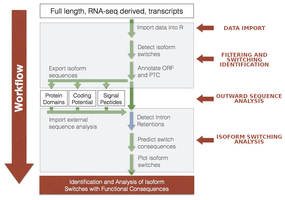
In this training, the IsoformSwitchAnalyzeR stage is divided in four steps:
Data import: import into IsoformSwitchAnalyzeR the transcription-level expression measurement dataset generated by Stringtie. This step also requires to import the GTF annotation file and the transcriptome.
Pre-processing step: non-informative gene/isoforms are removed from the datasets and differentially isoform usage analysis with DEXSeq. Once the IS have been found, the corresponding nucleotide and aminoacid sequences are extracted.
Outward sequence analysis: The sequences obtained in the previous step are used in order to evaluate their coding potential and the motifs that they contain by using two different tools: PfamScan and CPAT.
Isoform splicing analysis: The final step involves importing and incorporating the results of the external sequence analysis, identifying intron retention, predicting functional consequences and generating the reports.
Comment: On the alternative splicing concept
In accordance with the IsoformSwitchAnalyzeR developers, in this training the concept of alternative splicing englobes both alternative splicing (AS), alternative transcription start sites (ATSS) as well as alternative transcription start sites (ATTS).
Figure 11: IsoformSwitchAnalyzeR workflow scheme. The individual steps are indicated by arrows. Please note the boxes marked with “outward sequence analysis” requires to run a set of different tools. Adapted from IsoformSwitchAnalyzeR viggette.
Now, we can start with the IS analysis.
Split collection between the 2 conditions
We will generate 2 collections from the Stringtie output, one with the cancer samples and one with the healthy samples.
Hands-on: Task description
Extract element identifiersTool: toolshed.g2.bx.psu.edu/repos/iuc/collection_element_identifiers/collection_element_identifiers/0.0.2 with the following parameters:
“Dataset collection”: StringTie on collection N: transcript-level expression measurements
Search in textfilesTool: toolshed.g2.bx.psu.edu/repos/bgruening/text_processing/tp_grep_tool/1.1.1 with the following parameters:
“Select lines from”: Extract element identifiers on data N (output of Extract element identifierstool)
“that”: Match
“Regular Expression”: Cancer
Filter collecionTool: FILTER_FROM_FILE with the following parameters:
“Input collection”: StringTie on collection N: transcript-level expression measurements
“How should the elements to remove be determined”: Remove if identifiers are ABSENT from file
“Filter out identifiers absent from”: Search in textfiles on data N (output of Search in textfilestool)
Rename both collections Transcripts Health and Transcripts Cancer.
Import data into IsoformSwitchAnalyzeR
The first step of the IsoformSwitchAnalyzeR pipeline is to import the required datasets.
Comment: Salmon as source of transcript-expression data
In addition of Stringtie, it is possible to import dada from SALMON. The main advantage of Salmon over StringTie for isoform differential expression analysis is its speed and computational efficiency, while achieving similar accuracies when analyzing known transcripts. However, StringTie is considered a better alternative if we are interested in novel transcript features.
Hands-on: Task description
IsoformSwitchAnalyzeRTool: toolshed.g2.bx.psu.edu/repos/iuc/isoformswitchanalyzer/isoformswitchanalyzer/1.20.0+galaxy0 with the following parameters:
“Tool function mode”: Import data
In “1: Factor level”:
“Specify a factor level, typical values could be ‘tumor’ or ‘treated’“: Cancer
param-collection“Transcript-level expression measurements”: Transcripts Cancer
In “2: Factor level”:
“Specify a factor level, typical values could be ‘tumor’ or ‘treated’“: Health
param-collection“Transcript-level expression measurements”: Transcripts Health
It generates a switchAnalyzeRlist object that contains all relevant information about the isoforms involved in isoform swtches, such as each comparison of an isoform between conditions.
Pre-processing step
Once the datasets have been imported into a RData file, we can start with the pre-processing step. In order to enhace the reliability of the downstream analysis, it is important to remove the non-informative genes/isoforms (e.g. single isoform genes and non-expressed isoforms).
After the pre-processing, IsoformSwitchAnalyzieR performs the differential isoform usage analysis by using DESXSeq, which despite originally designed for testing differential exon usage, it has demonstrated to perform exceptionally well for differential isoform usage.DEXSeq uses generalized linear models to assess the significance of observed differences in isoform usage values between conditions, taking into account the biological variation between replicates (Anders and Reyes 2017).
Comment: Difference in isoform fraction contept
IsoformSwitchAnalyzeR measures isoform usage vian isoform fraction (IF) values which quantifies the fraction of the parent gene expression originating from a specific isoform, (calculated as isoform_exp / gene_exp). Consequently, the difference in isoform usage is quantified as the difference in isoform fraction (dIF) calculated as IF2 - IF1, and these dIF are used to measure the effect size (Kristoffer 2017).
IsoformSwitchAnalyzeR uses two parameters to define a significant IS:
Alpha: the FDR corrected P-value (Q-value) cutoff.
dIFcutoff: the minimum (absolute) change in isoform usage (dIF).
This combination is used since a Q-value is only a measure of the statistical certainty of the difference between two groups and thereby does not reflect the effect size which is measured by the dIF values (Kristoffer 2017).
Comment: Isoform or gene resolution analysis?
Despite IsoformSwitchAnalyzeR supports both isoform and gene resolution analysi, it is recommended to tu use the isoform-level analysis. The reason is that since the analysis is restricted to genes involved in IS, gene-level analysis is conditioned by higher false positive rates.
IsoformSwitchAnalyzeRTool: toolshed.g2.bx.psu.edu/repos/iuc/isoformswitchanalyzer/isoformswitchanalyzer/1.20.0+galaxy0 with the following parameters:
“Tool function mode”: Analysis part one: Extract isoform switches and their sequences
param-file“IsoformSwitchAnalyzeR R object”: SwitchList (output of IsoformSwitchAnalyzeRtool)
Comment: Reduce to switch genes option
An important argument is the ‘Reduce to switch genes’ option. When enabled, it will reduce/subset of genes to those which each contains at least one differential used isoform, as indicated by the alpha and dIFcutoff cutoffs. This option ensures the rest of the workflow runs significantly faster since isoforms from genes without IS are not analyzed.
Outward sequence analysis
The next step is to use to use generated FASTA files corresponding to the aminoacid and nucleotide sequences to perform the external analysis tools. In that case, we will use PfamScan for predicting protein domains and CPAT predicting the coding potential. This information will be integrated in the downstream analysis.
Comment: Additional sequence analysis tools
Note that IsoformSwitchAnalyzeR allows to integrate additional sources, such as prediction of signal peptides (SignalP) and intrinsically disordered regions (IUPred2AIUPred2A or NetSurfP-2). However, those tools are not currenly available in Galaxy, so for this reason we will not make use of them. You can find more information in the IsoformSwitchAnalyzeR viggette.
Protein domain identification with PfamScan
PfamScan is an open-source tool developed by the EMBL-EBI for identifying protein motifs. It allows to search FASTA sequences against Pfam HMM libraries. This tool requires three input datasets:
Pfam-A HMMs in an HMM library searchable with the hmmscan program: Pfam-A.hmm.gz
Pfam-A HMM Stockholm file associated with each HMM required for PfamScan: Pfam-A.hmm.dat.gz
Active sites dataset: active_sites.dat.gz
Comment: Pfam database
Pfam is a collection of multiple sequence alignments and profile hidden Markov models (HMMs). Each Pfam profile HMM represents a protein family or domain. Pfam families are divided into two categories, Pfam-A and Pfam-B.
Pfam-A is a collection of manually curated protein families based on seed alignments, and it is the primary set of families in the Pfam database. Pfam-B is an automatically generated supplement to Pfam-A, containing additional protein families not covered by Pfam-A, derived from clusters produced by MMSeqs2. For most applications, Pfam-A is likely to provide more accurate and interpretable results, but using Pfam-B can be helpful when no Pfam-A matches are found.
Hands-on: Domain identification with PfamScan
PfamScanTool: toolshed.g2.bx.psu.edu/repos/bgruening/pfamscan/pfamscan/1.6+galaxy0 with the following parameters:
param-file“Protein sequences FASTA file”: aminoacid sequences (output of IsoformSwitchAnalyzeRtool)
param-file“Pfam-A HMM library”: Pfam-A.hmm.gz
param-file“Pfam-A HMM Stockholm file”: Pfam-A.hmm.dat.gz
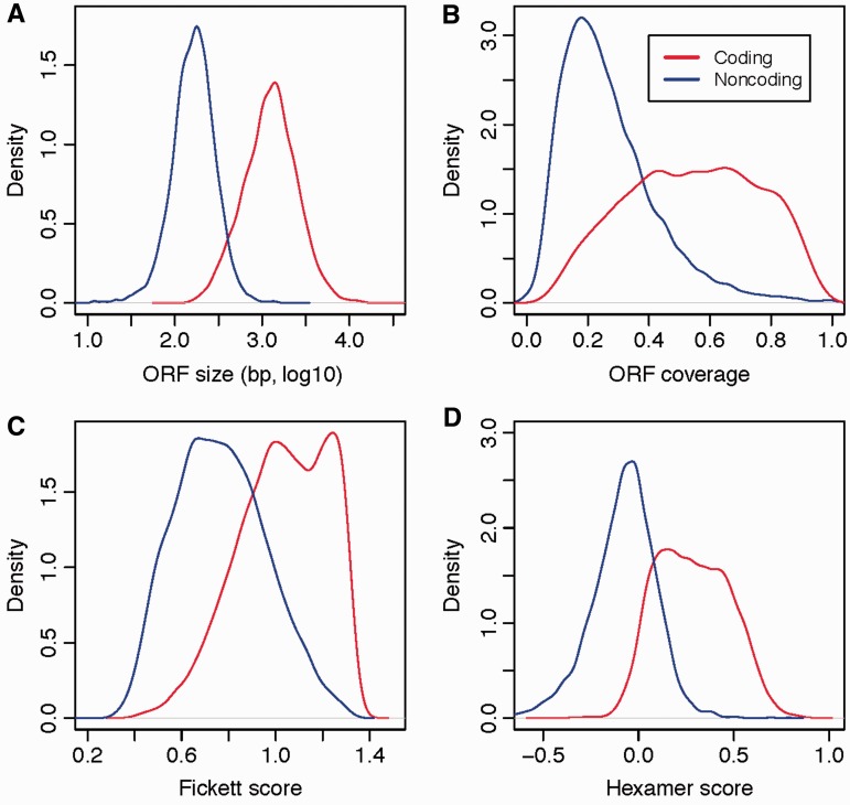
CPAT (Coding-Potential Assessment Tool ) is an open-source alignment-free tool, which uses logistic regression to distinguish between coding and noncoding transcripts on the basis of four sequence features. To achieve this goal, CPAT computes the following four metrics: maximum length of the open reading frame (ORF), ORF coverage, Fickett TESTCODE and Hexamer usage bias.
Each of those metrics is computed from a set of known protein-coding genes and another set of non-coding genes. CPAT will then builds a logistic regression model using theses as predictor variables and the “protein-coding status” as the response variable. After evaluating the performance and determining the probability cutoff, the model can be used to predict new RNA sequences (Wang et al. 2013).
CPAT makes use of for predictior variables for performing the coding-potential analysis. The figure 10 shows the scoring distribution between coding and noncoding transcripts for the four metrics.
Figure 12: Example of score distribution between coding (red) and noncoding (blue) sequences for the four CPAT metrics. The different subplots correspond to ORF size (A), ORF coverage (B), Fickett score (TESTCODE statistic) (C) and hexamer usage bias measured by log-likelihood ratio (D). Source: Wang et al., 2013
The maximum length of the ORF (fig. 10,A) is one of the most fundamental features used to distinguish ncRNA from messenger RNA because a long putative ORF is unlikely to be observed by random chance in noncoding sequences.
The ORF coverage (fig. 10, B) is the ratio of ORF to transcript lengths. This feature has demonstrated to have good classification power, and it is highly complementary to, and independent of, the ORF length (some large ncRNAs may contain putative long ORFs by random chance, but usually have much lower ORF coverage than protein-coding RNAs).
The Fickett TESTCODE (fig. 10, C) distinguishes protein-coding RNA and ncRNA according to the combinational effect of nucleotide composition and codon usage bias. It is independent of the ORF, and when the test region is ≥200 nt in length (which includes most lncRNA), this feature alone can achieve 94% sensitivity and 97% specificity.
Finally, the fourth metric is the hexamer usage bias (fig. 10, D), determines the relative degree of hexamer usage bias in a particular sequence. Positive values indicate a coding sequence, whereas negative values indicate a noncoding sequence.
Hands-on: Coding prediction with CPAT
CPATTool: toolshed.g2.bx.psu.edu/repos/bgruening/cpat/cpat/3.0.4+galaxy0 with the following parameters:
param-file“Query nucletide sequences”: Nucleotide sequences (output of IsoformSwitchAnalyzeRtool)
No ORF: Sequence IDs or BED entries with no ORF found. Should be considered as non-coding.
ORF probabilities (TSV): ORF information (strand, frame, start, end, size, Fickett TESTCODE score, Hexamer score) and coding probability.
ORF best probabilities (TSV): The information of the best ORF. This file is a subset of the previous one.
ORF sequences (FASTA): The top ORF sequences (at least 75 nucleotides long) in FASTA format.
For the downstream analysis, we will use only the ORF best probabilities, but it will require some minor modifications in order to be used as input to IsoformSwitchAnalyzeR.
Hands-on: Required format modifications on CPAT output
Remove beginningTool: Remove beginning1 with the following parameters:
“Remove first”: 1
param-file“From”: ORF best probabilities (TSV) (output of CPATtool)
Text reformattingTool: toolshed.g2.bx.psu.edu/repos/bgruening/text_processing/tp_awk_tool/1.1.2 with the following parameters:
param-file“File to process”: output of Remove beginning
Concatenate datasetsTool: cat1 with the following parameters:
param-file“Concatenate Dataset”: CPAT_header.tab
In “Dataset”:
Click in “Insert Dataset”
In “1: Dataset”:
param-file“Select”: output of Text reformatting
Isoform switching analysis
Once the expression data has been integrated and the required auxiliar information has been generated, we can start with the final stage of the analysis. IsoformSwitchAnalyzeR will extract the isoforms with significant changes in their isoform usage and the isoform, that compensate for the changes. Then, those isoforms are classified according to their contribution to gene expression (determinated by the dIF values). Finally, the isoforms with increased contribution (dIF values larger than the dIFcutoff) are compared in a pairwise manner to the isoforms with negative contribution.
IsoformSwitchAnalyzeR allows two analysis modes:
Analysis of individual IS
Genome-wide analysis of IS
In the next sections we will illustrate both different use-cases.
Gene-specific isoform switching analysis
The gene-specific mode is interesting for those experimental designs which aim to evaluate a pre-selected set of genes of interest. For this purpose, we can analyze the expression pattern of the gene RGMB (repulsive guidance molecule BMP co-receptor b), whose aberrant expression is suggested to be associated with cancer cell proliferation through the BMP pathway (Shi et al. 2015).
IsoformSwitchAnalyzeRTool: toolshed.g2.bx.psu.edu/repos/iuc/isoformswitchanalyzer/isoformswitchanalyzer/1.20.0+galaxy0 with the following parameters:
“Tool function mode”: Analysis part two: Plot all isoform switches and their annotation
param-file“IsoformSwitchAnalyzeR R object”: switchList (output of IsoformSwitchAnalyzeRtool part 1)
“Analysis mode”: Analyze specific gene
“Gene name”: RGMB
“Include prediction of coding potential information”: CPAT
param-file“CPAT result file”: Concatenate datasets on data ... (output of Concatenate datasetstool)
“Include Pfam information”: Enabled
param-file“Include Pfam results (sequence analysis of protein domains)”: PfamScan on data ... (output of PfamScantool)
“Include SignalP results”: Disabled
“Include prediction of intrinsically disordered Regions (IDR) information”: Disabled
Let’s have a look at the generated plot (fig. 13).
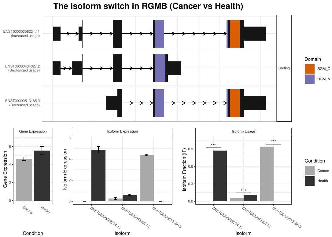
Figure 13: RGMB isoform expression profile plot. The plot integrates isoform structures along with the annotations, gene and isoform expression and isoform usage including the result of the isoform switch test.
In that case, we can appreciate that despite differences in overall gene expression is not statistically significant between health and cancerous tissues, there exists statistically significant IS: the isoform ENST00000308234.11, which encodes the 478 aminoacid Repulsive guidance molecule BMP co-receptor b protein is repressed in cancer; on the other hand, the isoform ENST00000513185.3, which encodes the 437 aminoanid Repulsive guidance molecule B is induced.
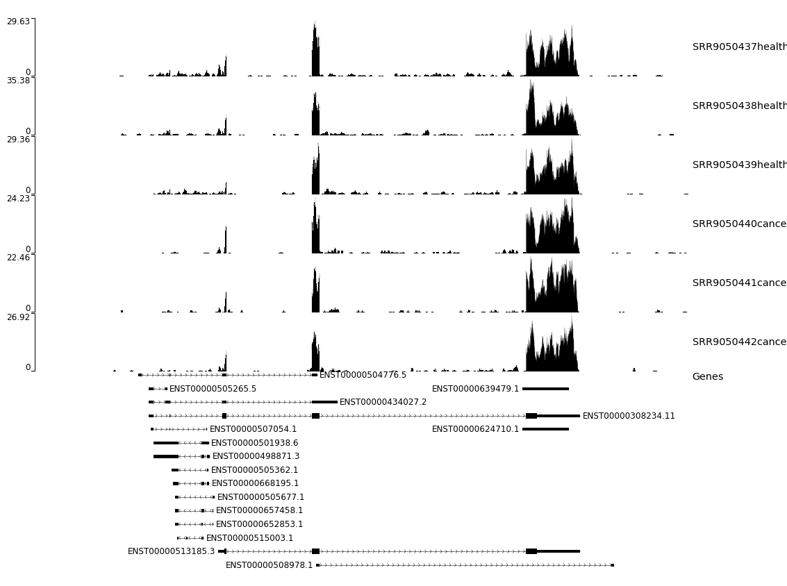
We will try to confirm this IS by visualising the coverage on this gene and more precisely on the region which is different between the two isoforms. We will take advantage of the coverage we generated with STAR and use a software called pyGenomeTracks
Hands-on: Check isoform switching with pyGenometracks from STAR coverage
“Region of the genome to limit the operation”: chr5:98,762,495-98,803,294
In “Include tracks in your plot”:
param-repeat“Insert Include tracks in your plot”
“Choose style of the track”: Bedgraph track
“Plot title”: You need to leave this field empty so the title on the plot will be the sample name.
param-collection“Track file(s) bedgraph format”: Select RNA STAR on collection N: Coverage Uniquely mapped strand 1.
“Minimum value”: 0
“height”: 3
“Show visualization of data range”: Yes
“Include spacer at the end of the track”: 1
param-repeat“Insert Include tracks in your plot”
“Choose style of the track”: Gene track / Bed track
“Plot title”: Genes
param-file“Track file(s) bed or gtf format”: Select gencode.v43.annotation.gtf.gz
“height”: 10
“Put all labels inside the plotted region”: Yes
“Bed style”: UCSC
“Configure other bed parameters”:
“When using gtf as input”:
“attribute to use as label”: transcript_id
Let’s have a look at the plot generated by pyGenometracks (fig. 14).
Figure 14: pyGenometracks isoform visualization. The plot integrates coverage information of the different RGMB gene isoform structures along with the annotations.
IsoformSwitchAnalyzer genome-wide analysis
A genome-wide analysis is both useful for getting an overview of the extent of IS as well as discovering general patterns. In this training we will perform three different summaries/analyses for both the analysis of AS and IS with predicted consequences:
Global summary statistics for summarizing the number of switches with predicted consequences and the number of splicing events occurring in the different comparisons.
Analysis of splicing/consequence enrichment for analyzing whether a particular consequence/splice type occurs more frequently than the opposite event.
Analysis of genome-wide changes in isoform usage for analyzing the genome-wide changes in isoform usage for all isoforms with particular opposite pattern events.
Comment: Difference in isoform fraction
If an isoform has a significant change in its contribution to gene expression, there must per definition be reciprocal changes in one (or more) isoforms in the opposite direction, compensating for the change in the first isoform. Thus,the isoforms used more (positive dIF) can be compared to the isoforms used less (negative dIF) and by systematically identify differences annotation it is possible to identify potential function consequences of the IS event.
Hands-on: Isoform switch analysis
IsoformSwitchAnalyzeRTool: toolshed.g2.bx.psu.edu/repos/iuc/isoformswitchanalyzer/isoformswitchanalyzer/1.20.0+galaxy0 with the following parameters:
“Tool function mode”: Analysis part two: Plot all isoform switches and their annotation
param-file“IsoformSwitchAnalyzeR R object”: switchList (output of IsoformSwitchAnalyzeRtool part 1)
“Analysis mode”: Full analysis
“Include prediction of coding potential information”: CPAT
param-file“CPAT result file”: Concatenate datasets on data ... (output of Concatenate datasetstool)
“Include Pfam information”: Enabled
param-file“Include Pfam results (sequence analysis of protein domains)”: output (output of PfamScantool)
“Include SignalP results”: Disabled
“Include prediction of intrinsically disordered Regions (IDR) information”: Disabled
Comment: Only significantly differential isoforms
A more strict analysis can be performed by enabling the Only significantly differential used isoforms option, which causes to only consider significant isoforms meaning the compensatory changes in isoform usage are ignored unless they themselves are significant.
It generates five tabular files with the results of the different statistical analysis:
Splicing summary: values of the different splicing events
Splicing enrichment: results of enrichment statistical analysis for the different splicing events.
Consequences summary: values of global usage of IS
Consequences enrichment: results of enrichment statistical analysis for the different functional consequences.
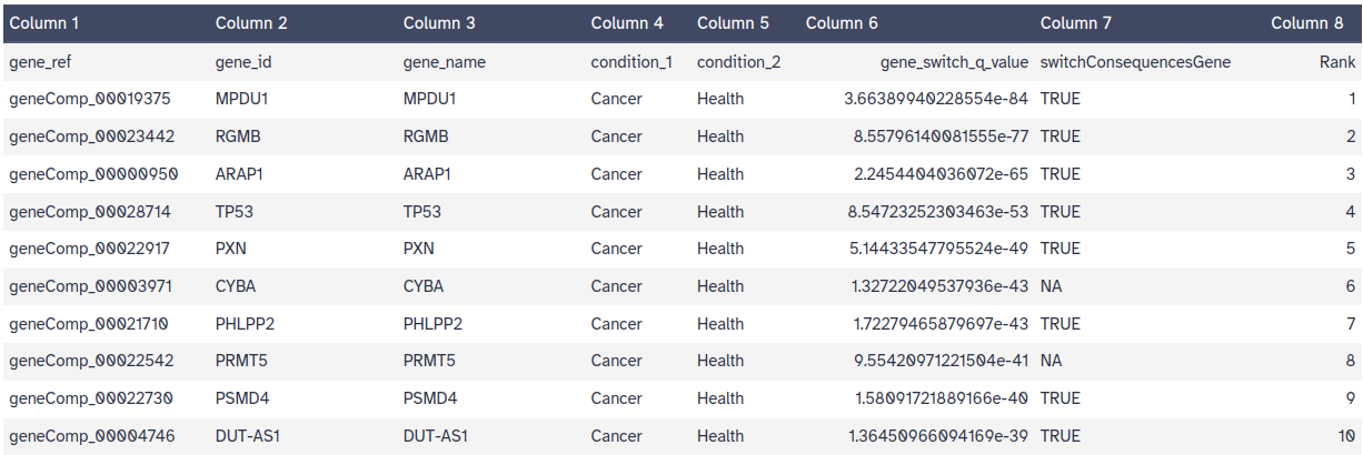
Switching gene/isoforms: list of genes with statistically significant isoform swiching between conditions (table 1). The switches are ranked (by p-value or switch size).
Question
What are the the top three IS events (as defined by alpha and dIFcutoff)?
The top three genes are MPDU1, RGMB and ARAP1 (fig. 15).
Figure 15: Switching gene/isoform dataset.
In addition, it provides a RData object and three collections of plots: IS events with predicted functional consequences, IS without predicted functional consequences and genome-wide plots.
Analysis of splicing enrichment
In this section we will assess whether there are differences with respect to the type of AS event .
Comment: Interpretation of splicing events
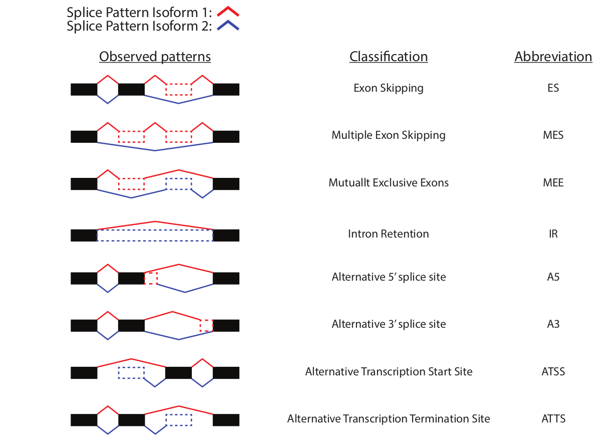
The events are classified by comparing the splicing patterns with a hypothetical pre-RNA generated by combining all the exons (fig. 16).
Figure 16: Splicing patterns diversity. The observed splice patterns (left column) of two isoforms compared as indicated by the color of the splice patterns. The corresponding classification of the event (middle column) and the abreviation used (right column).
ES: Exon Skipping. Compared to the hypothetical pre-RNA a single exon was skipped in the isoform analyzed.
MEE: Mutually exclusive exon. Special case were two isoforms form the same gene contains two mutually exclusive exons and which are not found in any of the other isoforms from that gene.
MES: Multiple Exon Skipping. Compared to the hypothetical pre-RNA multiple consecutive exon was skipped in the isoform analyzed.
IR: Intron Retention. Compared to the hypothetical pre-RNA an intron was retained in the isoform analyzed.
A5: Alternative 5’end donor site. Compared to the hypothetical pre-RNA an alternative 5’end donor site was used. Since it is compared to the pre-RNA, the donor site used is per definition more upstream than the pre-RNA (the upstream exon is shorter).
A3: Alternative 3’end acceptor site. Compared to the hypothetical pre-RNA an alternative 3’end acceptor site was used. Since it is compared to the pre-RNA, the donor site used is per definition more downstream than the pre-RNA (the downstream exon is shorter).
ATSS: Alternative Transcription Start Sites. Compared to the hypothetical pre-RNA an alternative transcription start sites was used. Since it is compared to the pre-RNA, the ATSS site used is per definition more downstream the the pre-RNA.
ATTS: Alternative Transcription Termination Sites. Compared to the hypothetical pre-RNA an alternative transcription Termination sites was used. Since it is compared to the pre-RNA, the ATTS site used is per definition more upstream than the pre-RNA.
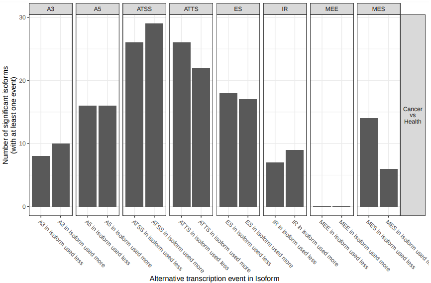
First, we will start analyzing the total number of splicing events (fig. 17).
Figure 17: Analysis of splicing enrichment. Number of isoforms significantly differentially used between cancer and health resulting in at least one splice event.
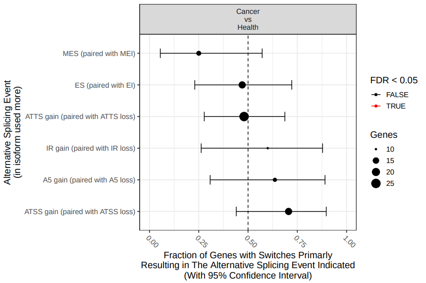
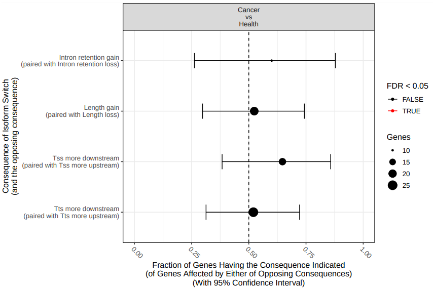
From the figure 17 , it can be hypothesised that some of the AS events are not equally used. To formally analyze this type of uneven AS, IsoformSwithAnalyzeR computes the fraction of events being gains (as opposed to loss) and perform a statistical analysis of this fraction by using a binomial test (fig. 18).
Figure 18: Comparison of differential splicing events. The fraction (and 95% confidence inter-val) of isoform switches (x-axis) resulting in gain of a specific alternative splice event (indicated by y axis) in the switch from health to cancer. Dashed line indicate no enrichment/depletion. Color indicate if FDR < 0.05 (red) or not (black).
According with the results (fig. 18), there are not statistically significant differences in specific splicing type events between both experimental conditions. However, this result is affected by the fact that we are using only a fraction of the total data (remember that we subsampled the origital datasets in order to speed up the analysis).
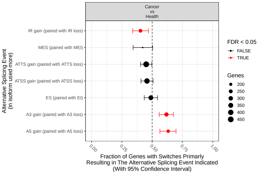
Comment: Results on original full-data
If we perform the analysis on the original datasets, there exist statistically significant differences in IS in three splicing patterns (fig. 19).
Figure 19: Comparison of differential splicing events. The fraction (and 95% confidence inter-val) of isoform switches (x-axis) resulting in gain of a specific alternative splice event (indicated by y axis) in the switch from health to cancer. Dashed line indicate no enrichment/depletion. Color indicate if FDR < 0.05 (red) or not (black).
According the results, there’s statistically significant gain of introl retention in cancer tissues. On the other hand, health tissues utilize alternative 3’ acceptor sites (A3) and alternative 5’ acceptor sites (A5) more than cancer tissues, when compared with the hyphotetical pre-RNA.
Analysis of consequence enrichment
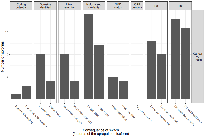
To analyze large-scale patterns in predicted IS consequences, IsoformSwitchAnalyzer computes all IS events resulting in a gain/loss of a specific consequence (e.g. protein domain gain/loss) when comparing cancer and ctrl (fig. 20). According the results some types of functional consequences seem to be enriched or depleted between health and tumoral samples (e.g. intron retention).
Figure 20: Analysis of consequence enrichment. Number of isoforms significantly differentially used between cancer and health resulting in at least one isoform switch consequence.
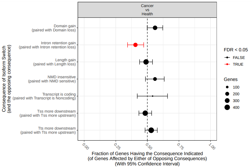
To assess this observation, a standard proportion test is performed (fig. 21). The results indicate that differences in intron retention between health and cancer samples is statistically significant).
Figure 21: Enrichment/depletion in isoform switches consequences. The x-axis shows the fraction (with 95% confidence interval) resulting in the consequence indicated by y axis, in the switches from cancer to control. Dashed line indicate no enrichment/depletion. Color indicate if FDR < 0.05 (red) or not (black).
According with the results (fig. 21), there are not statistically significant differences of IS consequences despite the apparent differentes in total event counts. However, as noted previously, in that case it is due to the small size of the datasets used.
Comment: Results on original full-data
Let’s have a look at the results corresponding to the complete original dataset analysis.
Figure 22: Enrichment/depletion in isoform switches consequences. The x-axis shows the fraction (with 95% confidence interval) resulting in the consequence indicated by y axis, in the switches from cancer to control. Dashed line indicate no enrichment/depletion. Color indicate if FDR < 0.05 (red) or not (black).
According with the results (fig. 22), the difference in intron retention is statistically significant; it means that the probability of a specific intron to remain unspliced in the mature mRNA in cancer is higher than in health tissues.
Question
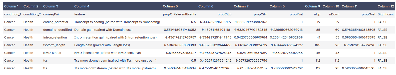
What is the adjusted P-value corresponding to the Intron retention gain/lost feature test?
The consequences enrichment tabular dataset includes the following columns:
conseqPair: The set of opposite consequences considered.
feature: Description of the functional consequence
propOfRelevantEvents: Proportion of total number of genes being of the type described in the feature column.
propCiLo: The lower boundary of the confidence interval.
propCiHi: The high boundary of the confidence interval.
propPval: The p-value associated with the null hypothesis.
nUp: The number of genes with the consequence described in the feature column.
nDown: The number of genes with the opposite consequence of what is described in the feature column.
propQval: The adjusted P-value resulting when p-values are corrected using FDR (BenjaminiHochberg).
This information can be found in the eighth column of the Consequences enrichment dataset (fig. 23).
Figure 23: Consequences enrichment table.
In that case, the adjusted P-value is 0.598.
Analysis of genome-wide changes in isoform usage
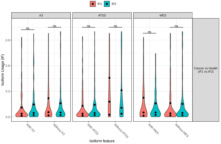
Finally, we will evaluate the genome-wide changes in isoform usage. This type of analysis allows to identify if differentes in splicing events are genome-wide or retricted to specific regions, and is particular interesting if the expected difference between conditions is large (fig. 24).
Figure 24: Genome-wide changes violin plot. The the dots in the violin plots above indicate 25th, 50th (median) and 75th percentiles.
As expected from the previous results, in that case there are not statistically significant genome-wide differences in splicing events.
Optional exercise: original data analysis
As additional activity, you can try to run the pipeline by using the original datasets. In that case we will make use of the Galaxy Workflow System, which will allow us to automatize the analysis by minimizing the number of required manual steps. We will start by importing the datasets from Zenodo.
Hands-on: Retrieve miRNA-Seq and mRNA-Seq datasets
Create a new history for this analsyis
Import the files from Zenodo:
Open the file galaxy-uploadupload menu
Click on Rule-based tab
“Upload data as”: Collection(s)
Copy the following tabular data, paste it into the textbox and press Build
Despite the large amount of RNA-seq data and computational methods available, isoform-based expression analysis is rare. Here we present a pipeline for the statistical identification and analysis of splicing event and IS events with predicted functional consequences.
Key points
Before starting RNA-seq data analysis, it is important to evaluate the quality of the samples by using RSeQC.
StringTie is a powerfull tool for gene isoform quantification and isoform switch analysis.
IsoformSwitchAnalyzeR allows to evaluate the statistical significance of isoform switch events in different conditions.
Further information, including links to documentation and original publications, regarding the tools, analysis techniques and the interpretation of results described in this tutorial can be found here.
References
Alt, F., 1980 Synthesis of secreted and membrane-bound immunoglobulin mu heavy chains is directed by mRNAs that differ at their 3\prime ends. Cell 20: 293–301. 10.1016/0092-8674(80)90615-7
Carninci, P., A. Sandelin, B. Lenhard, S. Katayama, K. Shimokawa et al., 2006 Genome-wide analysis of mammalian promoter architecture and evolution. Nature Genetics 38: 626–635. 10.1038/ng1789
Wang, E. T., R. Sandberg, S. Luo, I. Khrebtukova, L. Zhang et al., 2008 Alternative isoform regulation in human tissue transcriptomes. Nature 456: 470–476. 10.1038/nature07509
Kalsotra, A., and T. A. Cooper, 2011 Functional consequences of developmentally regulated alternative splicing. Nature Reviews Genetics 12: 715–729. 10.1038/nrg3052
Miura, K., W. Fujibuchi, and M. Unno, 2012 Splice isoforms as therapeutic targets for colorectal cancer. Carcinogenesis 33: 2311–2319. 10.1093/carcin/bgs347
Wang, L., S. Wang, and W. Li, 2012 RSeQC: quality control of RNA-seq experiments. Bioinformatics 28: 2184–2185. 10.1093/bioinformatics/bts356
Lu, B. X., Z. B. Zeng, and T. L. Shi, 2013 Comparative study of de novo assembly and genome-guided assembly strategies for transcriptome reconstruction based on RNA-Seq. Science China Life Sciences 56: 143–155. 10.1007/s11427-013-4442-z
Wang, L., H. J. Park, S. Dasari, S. Wang, J.-P. Kocher et al., 2013 CPAT: Coding-Potential Assessment Tool using an alignment-free logistic regression model. Nucleic Acids Research 41: e74–e74. 10.1093/nar/gkt006
Pertea, M., G. M. Pertea, C. M. Antonescu, T.-C. Chang, J. T. Mendell et al., 2015 StringTie enables improved reconstruction of a transcriptome from RNA-seq reads. Nature Biotechnology 33: 290–295. 10.1038/nbt.3122
Shi, Y., G.-B. Chen, X.-X. Huang, C.-X. Xiao, H.-H. Wang et al., 2015 Dragon (repulsive guidance molecule b, RGMb) is a novel gene that promotes colorectal cancer growth. Oncotarget 6: 20540–20554. 10.18632/oncotarget.4110
Veeneman, B. A., S. Shukla, S. M. Dhanasekaran, A. M. Chinnaiyan, and A. I. Nesvizhskii, 2015 Two-pass alignment improves novel splice junction quantification. Bioinformatics 32: 43–49. 10.1093/bioinformatics/btv642
Piovesan, A., M. Caracausi, F. Antonaros, M. C. Pelleri, and L. Vitale, 2016 GeneBase 1.1: a tool to summarize data from NCBI gene datasets and its application to an update of human gene statistics. Database 2016: baw153. 10.1093/database/baw153
Križanović, K., A. Echchiki, J. Roux, and M. Šikić, 2017 Evaluation of tools for long read RNA-seq splice-aware alignment (I. Birol, Ed.). Bioinformatics 34: 748–754. 10.1093/bioinformatics/btx668
Vitting-Seerup, K., and A. Sandelin, 2017 The Landscape of Isoform Switches in Human Cancers. Molecular Cancer Research 15: 1206–1220. 10.1158/1541-7786.mcr-16-0459
Bashyam, M. D., S. Animireddy, P. Bala, A. Naz, and S. A. George, 2019 The Yin and Yang of cancer genes. Gene 704: 121–133. 10.1016/j.gene.2019.04.025
Kovaka, S., A. V. Zimin, G. M. Pertea, R. Razaghi, S. L. Salzberg et al., 2019 Transcriptome assembly from long-read RNA-seq alignments with StringTie2. Genome Biology 20: 10.1186/s13059-019-1910-1
Bonnal, S. C., I. López-Oreja, and J. Valcárcel, 2020 Roles and mechanisms of alternative splicing in cancer — implications for care. Nature Reviews Clinical Oncology 17: 457–474. 10.1038/s41571-020-0350-x
Namba, S., T. Ueno, S. Kojima, K. Kobayashi, K. Kawase et al., 2021 Transcript-targeted analysis reveals isoform alterations and double-hop fusions in breast cancer. Communications Biology 4: 10.1038/s42003-021-02833-4
Glossary
AS
alternative splicing
IS
isoform switching
OCGs
oncogenes
TSGs
tumor supression genes
Feedback
Did you use this material as an instructor? Feel free to give us feedback on how it went.
Did you use this material as a learner or student? Click the form below to leave feedback.
Batut et al., 2018 Community-Driven Data Analysis Training for Biology Cell Systems 10.1016/j.cels.2018.05.012
@misc{transcriptomics-differential-isoform-expression,
author = "Cristóbal Gallardo and Lucille Delisle",
title = "Genome-wide alternative splicing analysis (Galaxy Training Materials)",
year = "",
month = "",
day = ""
url = "\url{http://0.0.0.0:4000/training-material/topics/transcriptomics/tutorials/differential-isoform-expression/tutorial.html}",
note = "[Online; accessed TODAY]"
}
@article{Hiltemann_2023,
	doi = {10.1371/journal.pcbi.1010752},
	url = {https://doi.org/10.1371%2Fjournal.pcbi.1010752},
	year = 2023,
	month = {jan},
	publisher = {Public Library of Science ({PLoS})},
	volume = {19},
	number = {1},
	pages = {e1010752},
	author = {Saskia Hiltemann and Helena Rasche and Simon Gladman and Hans-Rudolf Hotz and Delphine Larivi{\`{e}}re and Daniel Blankenberg and Pratik D. Jagtap and Thomas Wollmann and Anthony Bretaudeau and Nadia Gou{\'{e}} and Timothy J. Griffin and Coline Royaux and Yvan Le Bras and Subina Mehta and Anna Syme and Frederik Coppens and Bert Droesbeke and Nicola Soranzo and Wendi Bacon and Fotis Psomopoulos and Crist{\'{o}}bal Gallardo-Alba and John Davis and Melanie Christine Föll and Matthias Fahrner and Maria A. Doyle and Beatriz Serrano-Solano and Anne Claire Fouilloux and Peter van Heusden and Wolfgang Maier and Dave Clements and Florian Heyl and Björn Grüning and B{\'{e}}r{\'{e}}nice Batut and},
	editor = {Francis Ouellette},
	title = {Galaxy Training: A powerful framework for teaching!},
	journal = {PLoS Comput Biol} Computational Biology}
}
Congratulations on successfully completing this tutorial!
Galaxy Administrators: Install the missing tools
You can use Ephemeris's shed-tools install command to install the tools used in this tutorial.

 Cristóbal Gallardo
 Lucille Delisle
 Pavankumar Videm
Questions: